ENPH 253 2023 — Robots & Racing
<< click to return to front page
<< click to return to content page
- Project Management + Advanced Problem Solving
- Rapid Prototyping, Manufacturing + CAD (Onshape)
- Soldering, Electronics + PCB Design
- Troubleshooting (noise issues, signal integrity, software + hardware)
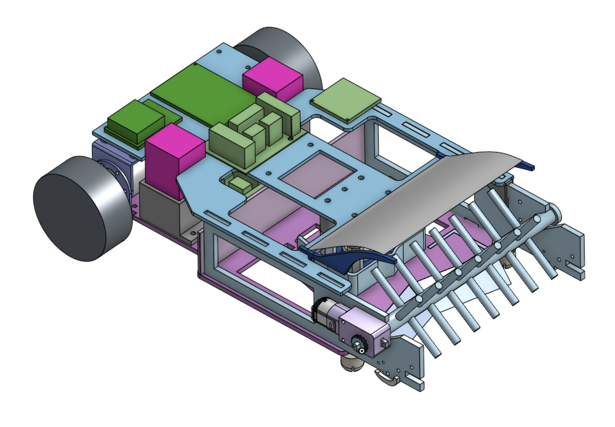
Over the 2023 Summer Term, spanning from July 4 to August 10, myself, Trevor Daykin, Amr Sherif, and Dhruv Arun were a team of 4 in the annual ENPH 253 robot competition. While the final robot iteration photos above are very similar, the path to this design was anything but straightforward. In this post, I outline my series of ideas, decisions, and work that led my team to success. In the end we were able to take home a 2nd-place finish.
ENPH 253, more commonly referred to as “robot summer”, is a course led by the Engineering Physics (ENPH) Project Lab at UBC. It is an autonomous robot competition which all 2nd year ENPH students must compete in to progress to their 3rd year of ENPH (ignoring the rare exceptions).
What’s special about this competition is that students design everything from scratch:
- Mechanical parts are all laser-cut, 3D-printed, waterjet sliced, and more.
- All electrical circuits must be soldered to and wired by hand. Moreover, no pre-made motor drivers can be purchased.
- Given the new theme each year, students must write new code.
Though the competition theme changes each year, the general structure of the course remains the same — teams consist of 4 students each, resulting in ~16 teams each year. Every team works ~6 weeks in the lab — which is open 10 A.M to 9 P.M every weekday — to design and rapidly prototype a fully autonomous robot capable of scoring “points”. In this year’s competition, which was a race between two robots at a time, points were obtained by picking up prizes, driving laps, and ziplining. After those 6 weeks complete, the competition is held in a world-cup style bracket system to ultimately declare a winner.
1. Competition Theme + Rules
Across previous years, the general competition idea was as follows: each team’s robot has a couple minutes on a set track filled with paths, collectibles, and obstacles. Each of these individual runs is called a “heat”. Increased travelling, collecting, and obstacle avoidance lead to more points scored in a heat. This sort of competition style never greatly rewarded speed, and so the final robots would slowly inch their way along the track, taking as much time as they could.
In a drastic change of theme, this year’s competition involved racing! Alongside paths, collectibles, and obstacles, now it was two robots on the same track at a time, in the same heat. Now, instead of one path going from start-to-end, it was a loop — faster robots who could complete more laps within a heat would gain more points.
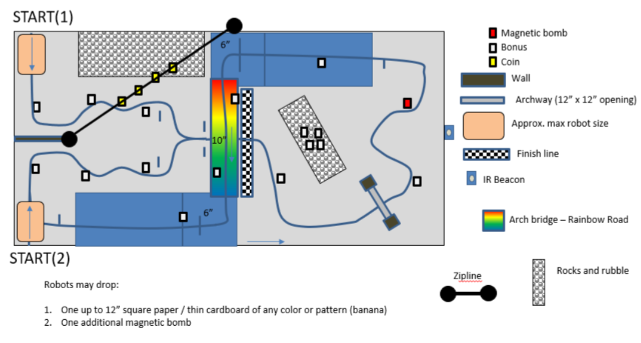
Here is a top-down view of the competition surface. The blue line is a tape track which robots can use to follow around the course, but they are not required to follow it. Both robots line up at either START(1) or START(2), and they would both begin running at the end of a countdown.
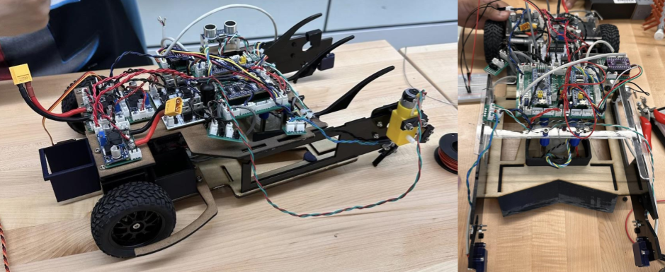
For a sense of scale, here’s our close-to-final robot driving under Rainbow Road from START(1).
A summary of important rules for the reader to be familiar with:
- Heats are 2 minutes long.
- Robot score points by picking up prize blocks (labelled “Bonus”) on the track, coins (labelled “Coin”) on the zipline, or by completing a lap. Blocks and coins are worth 1 point each, while a lap is worth 3.
- Regardless of START(1) or START(2), a lap is counted when a robot completes the following in order:
- crosses over the finish line
- goes up the ramp (blue, top right) and either jumps down on the left side of Rainbow Road, or loops around to START(2)
- travels under Rainbow Road from the left and crosses the finish line again
- A magnetic “bomb” is placed on the track, which has the same footprint as a regular Bonus / prize block. Each robot is also allowed to drop one extra bomb on the track at any time throughout the heat.
- Any robot that picks up a bomb, or tips it on its side has “detonated” the bomb, and they must restart, and also lose -3 points from any existing block / coin points.
2. Initial Team Ideas
While there were countless ways to go about scoring points, from the start we knew we wanted to take a very simple and routine approach. Almost immediately our team decided that we would follow the tape track and pick blocks up while avoiding bombs. Jumping off Rainbow Road, ziplining, or cutting over the rocks (to the right of the finish line) could be unpredictable, even if all software, mechanical, and electrical aspects were perfected.
Still, autonomously driving and picking up blocks, while somehow avoiding bombs is no easy task, especially when there’s another robot on the track. Here is the first design we set out to create:
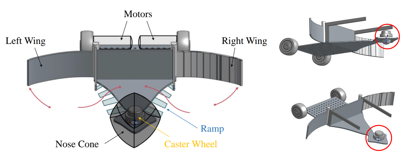
In this design, the robot would drive around the track, and blocks would make their way to the extended side wings, where they would be picked up. What was more of a statement in this design though, was how it would navigate.
There are two primary methods to turn a robot, shown below: [image source]

The first, called Ackerman-steering, is the type of steering you’d see in a car, where the back wheels drive at some speed, while the front wheels point in the direction of the turn.
The second, called differential-steering, is where the back wheels turn at different speeds to shift the car left or right. The diagram above shows four wheels, but it can also be done with two — one on each side — and some sort of pivoting caster (like a grocery cart’s front wheels). The caster we used is circled in red in the design images above.
Choosing an appropriate steering type was the first point of discussion for teams, because it determines the placement of motors, electronics, pickup mechanisms, and everything else around it. With the right geometry, mechanical design, and tuning, Ackermann steering is plenty faster than differential. This is likely why every team chose it — except us. Given the short time frame of the development period, we were certain that if spent more time perfecting Ackermann, which is harder to implement than differential, we may not have time to integrate block pickup and bomb avoidance.
Speaking of that, here is how our wings were going to integrate with our driving:
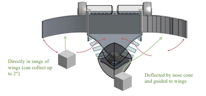
The idea was that, as the robot drove around, both blocks and bombs would make their way to the wings as the robot followed the tape. In the event of a block, the wings would fold up and push it into some catchment area as shown:
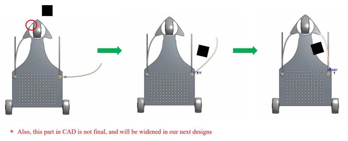
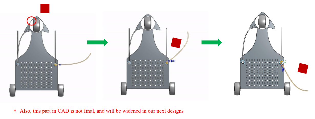
In the event of a bomb, the wings would instead fold back rather than closing forward. As the robot continues to drive forward, the bomb will slide along the edge of the wing and passively be pushed away to the side:
With all this in mind, we set out to get our first working chassis built.
3. Fundamentals and First Laps
To start, we decided to build a simple line-follower, which we could later adjust and add on to moving forward. To do so, I had to build our motor drivers, tape-following sensors, and microcontroller boards.
a) H-Bridge Motor Drivers
The H-Bridge is a relatively simple circuit used to control the polarity of the voltage across a load, in our case, a motor. Alongside having control over the speed by PWM, the H-bridge gives us control over the motor’s rotation direction. This is especially important in differential-steering, where in some cases one wheel must spin backward and the other forward to complete a sharp turn. Here is a simple dual H-bridge schematic of the motor boards on the robot.
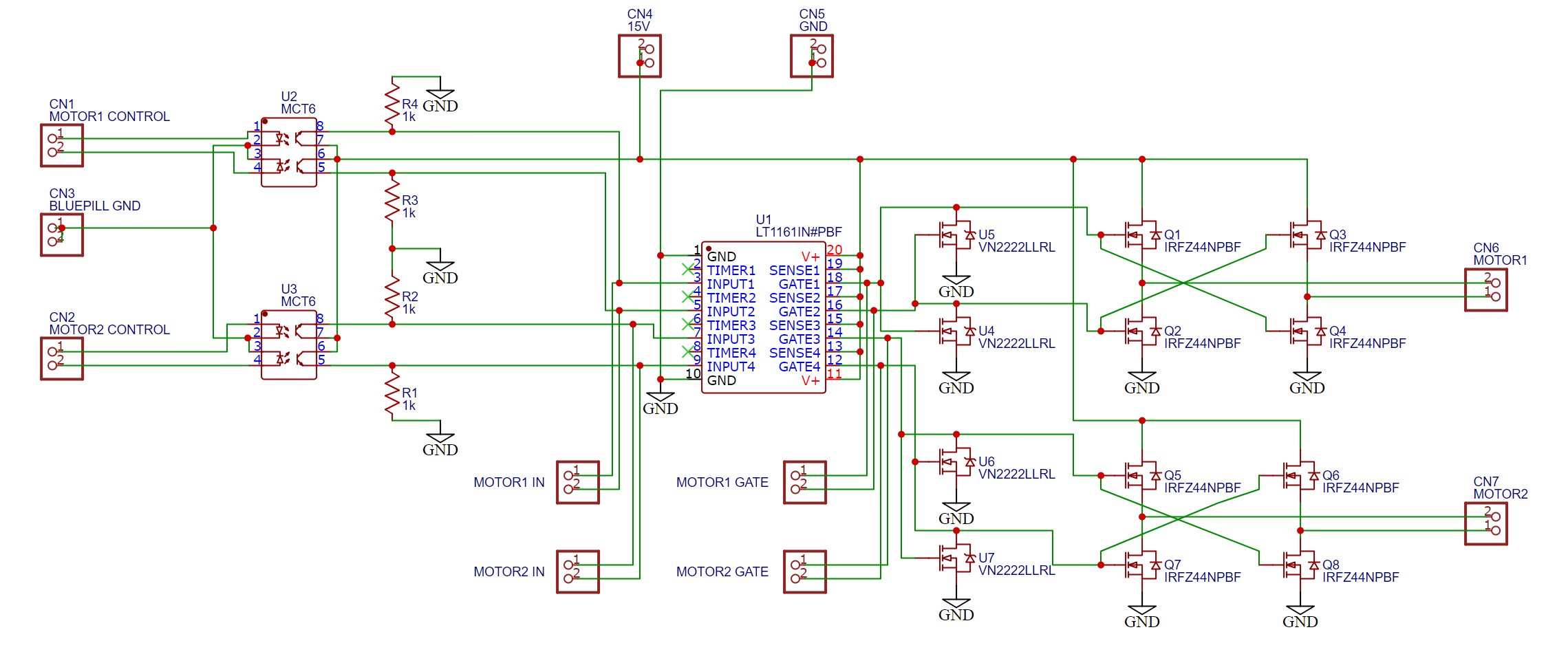
For those interested, here’s a step through of how the final H-Bridge board is derived.
With that understood, I put together our first dual H-Bridge driver on a 5 cm x 7 cm prototype board.
This is about as compact as it can get without making a PCB, just due to the large physical footprints of the MOSFETS and ICs.
Before I even started soldering however, it’s important to note that for this circuit (and every other one in the course), I started out by drawing out how all components would be laid out and wired together:
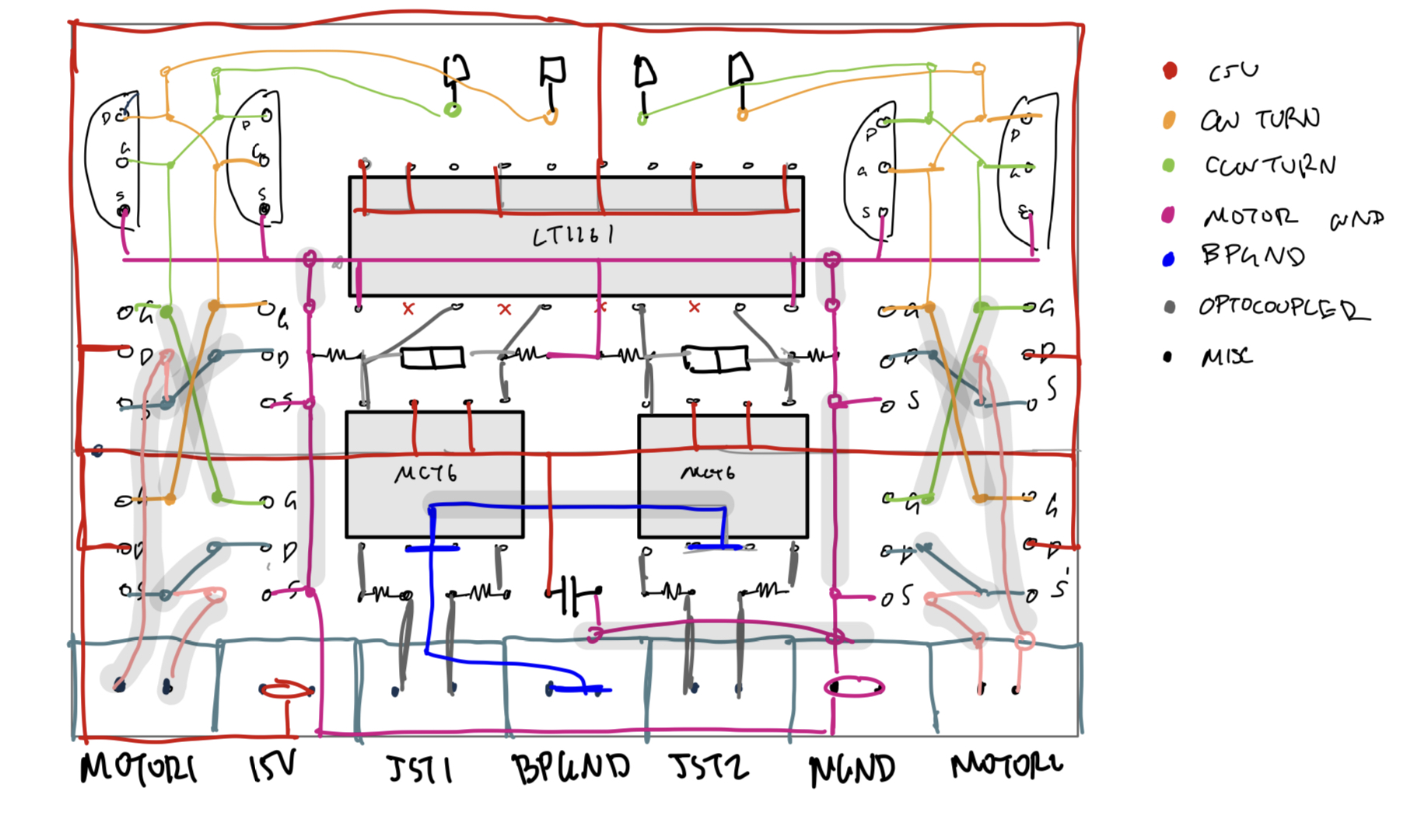
This still isn’t the full story, because some wires need to be specifically routed in order so that they don’t block the path of other wires, when the time comes to fit them in. So the next step was breaking down this image into a set of steps (like a Lego instruction manual).
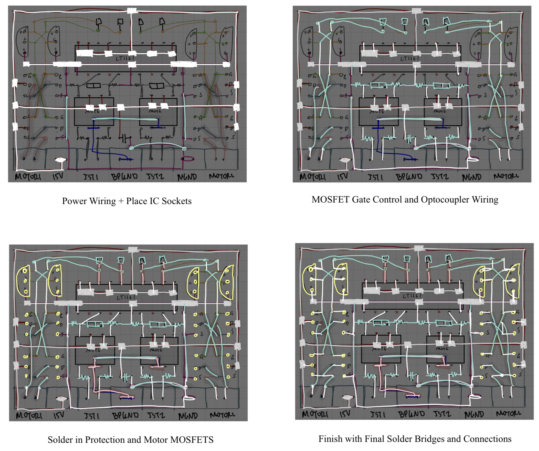
You can see how in the background of each step (slightly grayed out) is the original full image drawn which I showed just before. As we move through the instructions, it eventually becomes fully populated in the correct order.
Here’s the final hand-made board:
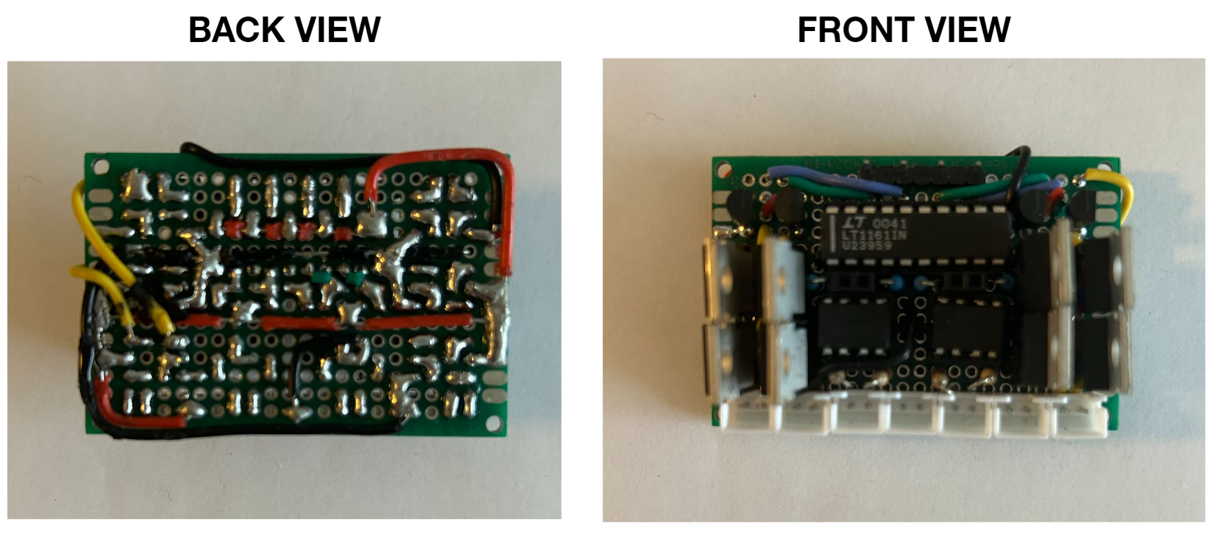
Trying to fit 2 H-Bridges like this into such a small footprint has diminishing returns, and I probably could have avoided half these steps if I had chosen a slightly-larger board (which wouldn’t have made a difference in the final robot). Moreover, it’s virtually impossible to troubleshoot a board like this due to the layers of wires routed over and under each other. Still, it was still pretty fun to make, and a good demonstration of my skills.
Soon after, I made a PCB-version of this board, which we used for the rest of the course:
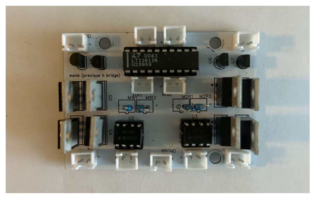
H-Bridge PCB Layout:
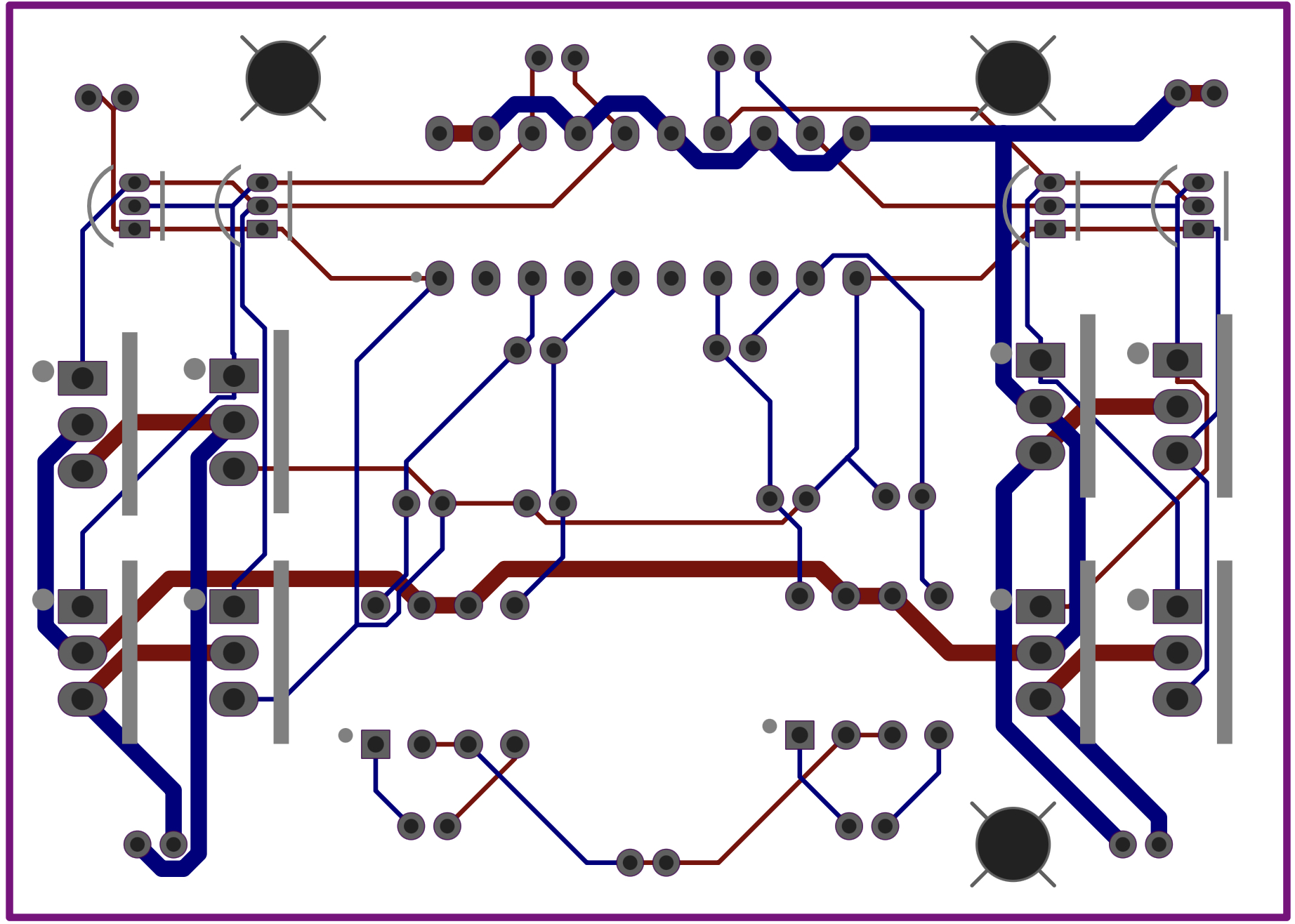
Layout-wise it’s almost identical to the hand-made one, but with mounting holes, probe points, and of course no visible wiring.
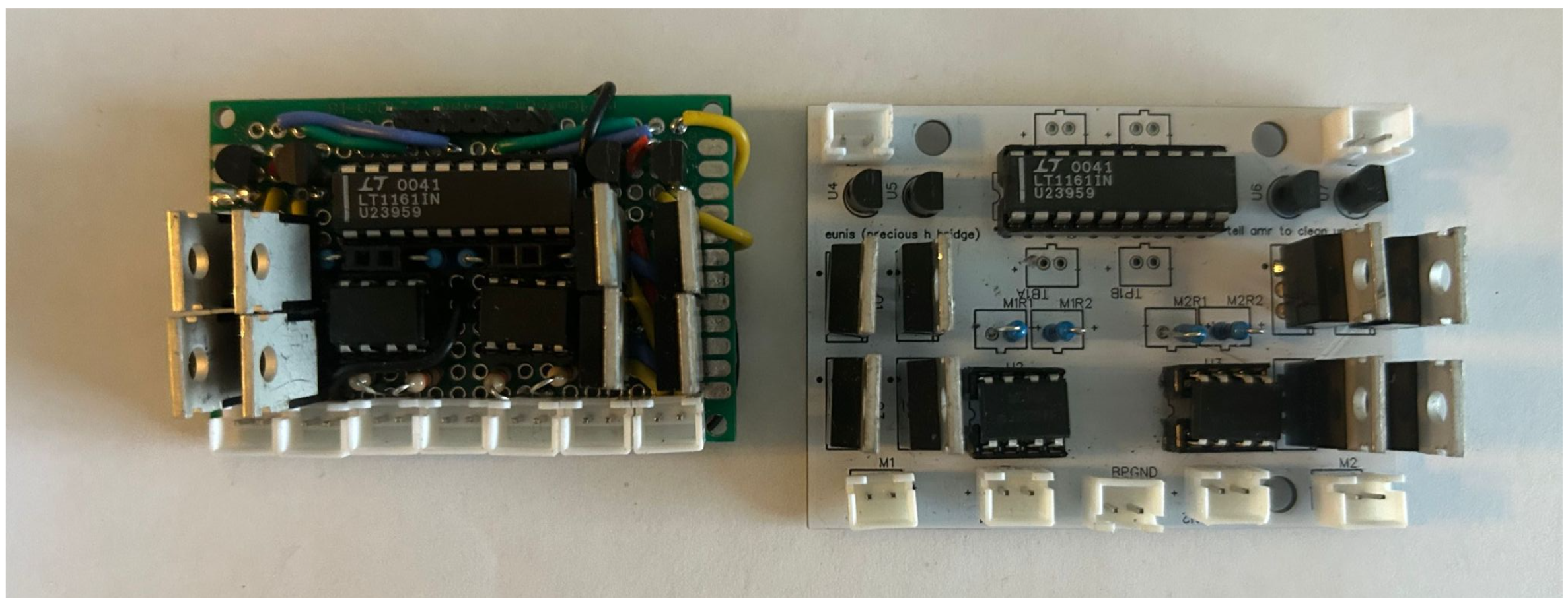
Putting the two boards side-by-side, the hand-made one is a little smaller, but then again it can’t be mounted without glue so I much more prefer the PCB.
b) Control Boards and Tape Following Sensors
Okay, that was a lot of rambling for just an H-Bridge. Luckily the microcontroller and tape following boards are much simpler. Here’s the unpopulated Blue-Pill/microcontroller board, and the tape sensor board.
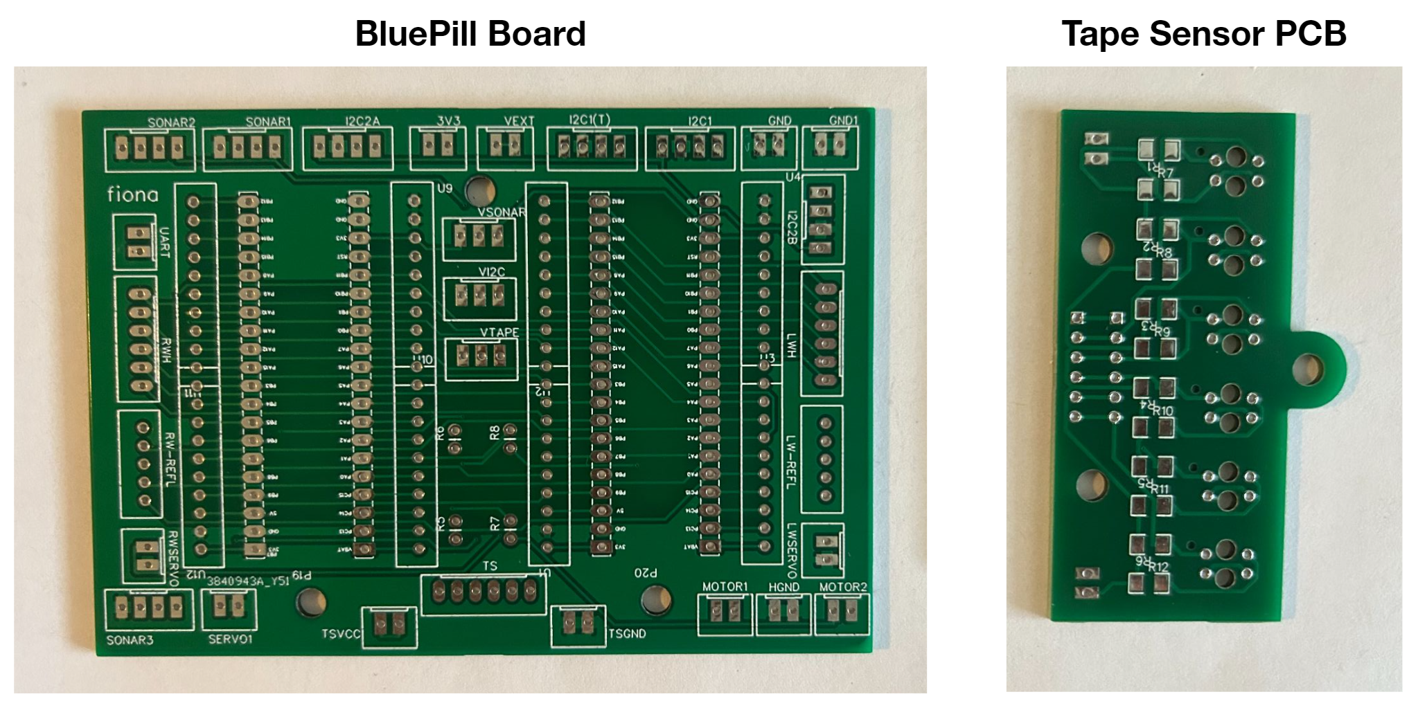
BP Board PCB Layout:
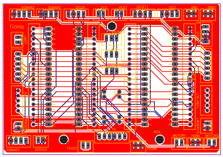
This is somewhat overkill and wasn’t really required in the end, but I designed this board pretty early on before any other sensor / peripheral decisions were made. So it just made sense to be safe and provide the possibility to house two microcontrollers. It has:
- x3 SONAR ports
- x4 I2C ports (two of them tied together if the microcontrollers need to talk to each other)
- x6 AIO available for tape sensors,
- x3 servo ports
- a UART port for serial monitor, power selection
- 2 2-wide PWM ports for two H-Bridges
- voltage level selectors for I2C, Sonar, and Tape Sensors
and leaves the remainder of the pins free for switches, LEDS, hall-sensors, and anything else.
For the tape-sensor board, Dhruv made the schematic and I made the PCB layout and soldered it together. It uses surface-mount resistors which was needed since the tape sensors sit very low to the ground. Here’s a video of it on a servo mount made by Trevor:
.gif)
c) PID Algorithm
The PID is probably the simplest part of code of the entire robot, but I wanted to share how I thought about converting tape-sensor data to an error function.
Instead of computing each sensor value and referencing a lookup table, I decided to treat each sensor value as a force on a seesaw. Then, simply let the displacement be the net torque on it! Of course, if the robot is completely off the line, then just reference the magnitude of the previous displacement to know whether you are too left, or too right.
That’s basically what I’m doing here — writing it in code is much simpler than doing it mathematically though. The key part is the which is simply the average. N is the location of each sensor and S is the associated sensor values.
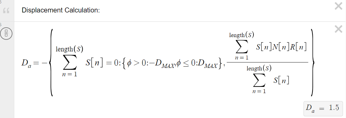
You can find the Desmos here, and play around with the , which is the displacement of the sensor array off the line. The purple line represents the error function value, and the dots are the sensor locations.
.gif)
One interesting way of doing it like this is it becomes convenient to introduce nonlinearities into the transfer function through the R[n] array. Trevor and I played around with this a little and found that a non-linear transfer function for differential steering can often result in smoother and more responsive driving than a linear one.
This makes intuitive sense for tape-following, because you don’t really care about minor deviations off the line, but once your tape sensors are close to leaving the line entirely, you now have a higher error to correct yourself quickly, or to take a sharp turn.
The final “non-traditional” part Trevor and I implemented was filtering the derivative of our error function, so that the PID equation is . To understand why, consider the following error function e(t), in red:
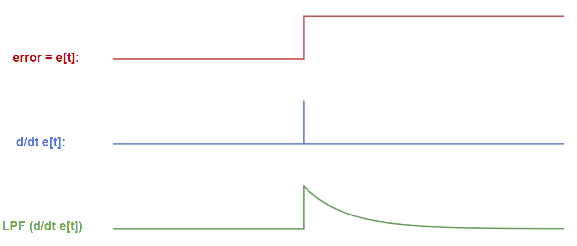
This error function simply means the robot’s displacement off the line has changed. It looks like a step rather than a smooth change because these signals are being processed inside the microcontroller, in thee discrete time domain.
If we then compute the almost-discrete-derivative as , we’d get an impulse, as shown in blue. This isn’t that useful because it means the derivative term in the PID equation only lasts for one loop iteration, which is on the order of s — that’s not nearly enough time for it to do much useful work. A solution to this is to low-pass filter (LPF) the differentiated error signal, shown in green. In an electrical context, this green signal represents the discharging of a capacitor, but instead we’re doing it in software using a first-order IIR filter:
Of course there are other ways to do this, and I guess you could choose any decaying function (maybe an average?). All that I’m trying to do is keep the effect of the derivative for longer, so that the term comes into play.
The motivation to try something like this is somewhat arbitrary, but we gave it a shot and it had a significant positive impact on the smoothness of the robot’s tape following at high speeds.
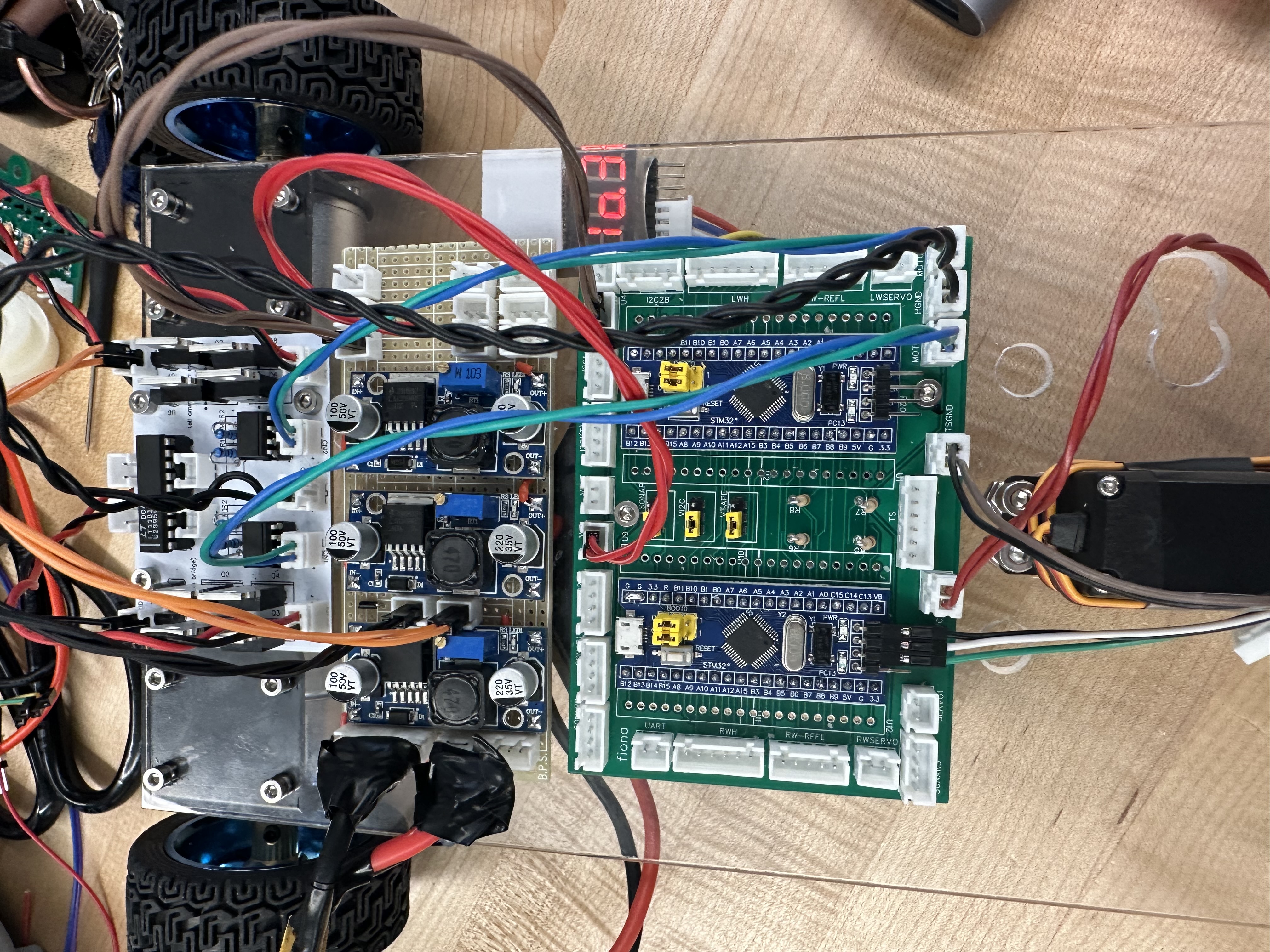
d) Final Run
With all the basics sorted, we put the motors, H-bridges, microcontrollers, tape-sensors, and PID code together for the first prototype. Here you can see one of the populated BP boards as well.
I’m really proud of the pace we were able to do this at, since we were the first team to get on the track and tape follow in the first week of the course.
.gif)
We fail on rainbow road since this was our first time testing, and the colors interfered with the tape sensor, but we all start somewhere!
3. Block Pickup and Redesigns
a) Side Wings:
After having spent some time on PID tuning and driving the base chassis around, it was time to start implementing the “wings” that would pick up the blocks themselves.
There isn’t much to talk about here — we mainly just changed some CAD, wrote some code, and re-assembled the same differential-driving chassis with some acrylic wings. Here’s a video of 1) blocks being picked up at a standstill, and 2) having the robot line follow the tape track while picking up 2 blocks.
.gif)
This is pretty nice and very close to our mock-ups shown in the design proposal … but it looks nothing like the final robot. Why is that?
It turns out that, unfortunately, the front nose cone often knocked blocks that were placed ahead of it on the track, before the wings even had a chance to come in contact with them. In all honesty, the video shown above was a pretty big fluke, and subsequent test runs did not go as well.
This was a huge surprise to us, because we had tested the possibility of blocks tipping or being pushed away by a front nose piece in the first week, using a simple cardboard nose and sliding it along the floor. And while there didn’t seem to be any problems then, actually running the robot made us realize that the jittery motion of the robot which is inherent to differential steering would “bat” the blocks far away from the tape track.
Geometrically, since differential steering steers from the back, tiny oscillations back and forth lead to large swinging of the front nose cone. Meanwhile, with Ackermann steering, the steering happens in the front, so the nose wiggles less.
To try and fix this, we tried redoing the nose cone shape, adding guards on the side, and dampening the front with foam, all to no avail. Does this mean we had made the wrong decision in the debate of Ackermann vs. Differential? Maybe, but it didn’t mean we had to switch. Since we put our block-pickup mechanism together pretty quickly, we decided to explore a different pickup mechanism which didn’t have this fault.
b) Front Roller
Several other teams had shown that a front, inwards-spinning roller also worked for picking up these light blocks. We decided to adopt that which led us to this re-design:
.jpg)
This looks like an entirely new build, but the back is essentially identical to the winged-robot, and we’ve just widened up the front so that we could connect some side panels which hold a light yellow motor and the spinner itself. The middle region between the front spinner and the back wheels is simply a hollow container for block storage.
4. Bomb Detection
In most previous competition, fake or “trap” objects placed on the track, which would penalize the team if their robot picked them up, had magnets embedded in them. In our competition, it was the “bomb”, with the same physical footprint as a regular gray prize block, but a magnet below one of the faces.
ENPH 253 provides hall-effect sensors which students can use to detect such magnetic fields, but they’re often very unreliable, need to placed in the right orientation, don’t work when they quickly pass by a magnet, and must be extremely close to the magnet source to detect anything.
My idea was to use a magnetometer, which is normally used to detect orientation with respect to the Earth’s magnetic field. These devices must be extremely sensitive, which means that as a prominent external magnet approaches it, it’s reading spikes greatly — which a microcontroller can detect! Before I get into the details, here it is in action:
.gif)
It doesn’t hesitate to pick up the gray (prize) blocks, but stops spinning as a bomb (black/orange) approaches. In fact, this detection happens from quite far away — it just looks slower than it is because the spinner has some inertia, and it takes time for it to come to a complete halt.
This is such a reliable and powerful method that it almost feels like cheating. But it’s not, which is why I wouldn’t be surprised if the future competition “trap” items must be detected in some other way.
How it works:
The magnetometer used is the QMC5883L/HMC5883L magnetometer, which communicates over I2C with the Blue-Pill. It passes through the following a first-order low-pass IIR + moving average filter chain, and then by checking if the derivative of that filter output is greater than a certain threshold, we can determine if a bomb is near / approaching.
With this configuration, each magnetometer has about a ~10 cm detection radius, but the width of the collection area was about ~16 cm, so we needed one on either side of the robot to cover the whole range:
They’re placed under and a little forward of the spinner, hidden behind the navy-blue 3d-printed covers to prevent damage:
With two identical magnetometers communicating over I2C however, they have the same bus address. We do have two microcontrollers, so we could connect one magnetometer its own Blue-Pill … instead we decided to use a TCA9584A I2C multiplexer controlled by one Blue-Pill to switch between the two sensors. With this configuration, each Blue Pill is completely independent — one handles the driving, and the other handles the bomb detection and the spinner.
I should mention that the detection range has a little bit of a dead-band in the center (just in front of where the two ranges above overlap), but as the front end of the robot oscillates, this dead-band is swept across back and forth several times, and the bomb is always detected.
5. Driving Zones
One nicety that Dhruv and I worked on was implementing driving zones, which allowed us to better tune for speed and PID values (if a region had more sharp turns, we could increase P). In principle this is really simple to implement — we just store a 2D array of P, I, D, speed, and motor frequency (for torque adjustments) values. Here are the zones …
_(1).png)
… and here’s that array:
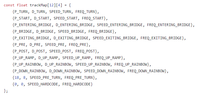
Each row in this array corresponds to which zone we’re in. Now we just use a long ugly list of if-statements to update our zones:
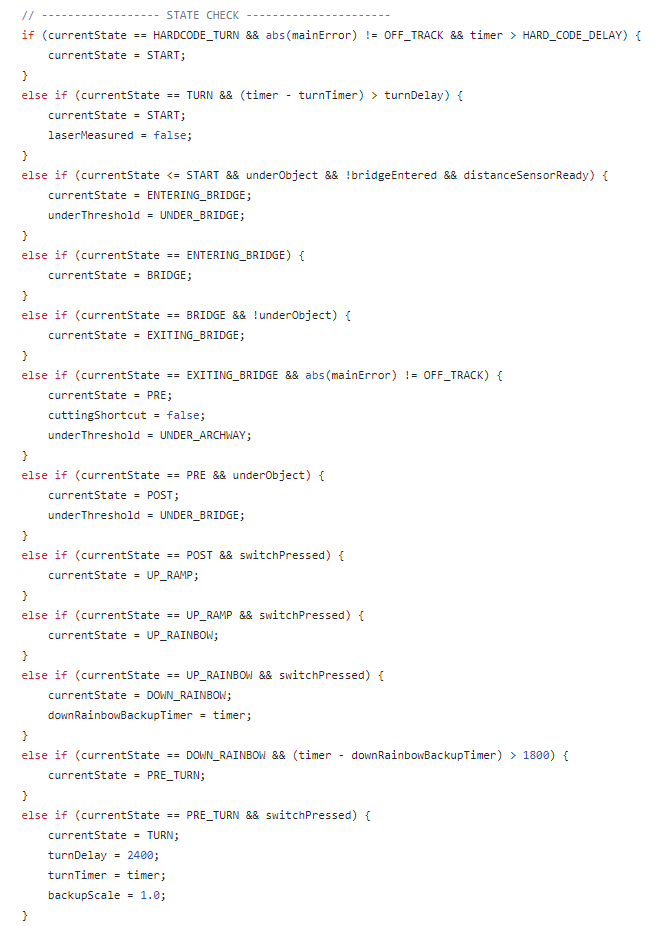
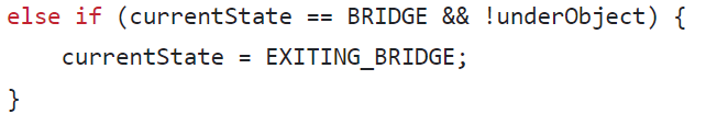
These if-statements increment our state around the track if a) we’re at some state, and b) if a physical marker on the track indicates a defined change that can only happen in that state. For example, if we’re in the BRIDGE state, but we see that we’re no longer under an object, we update the state to EXITING_BRIDGE:
a) Measuring Changes
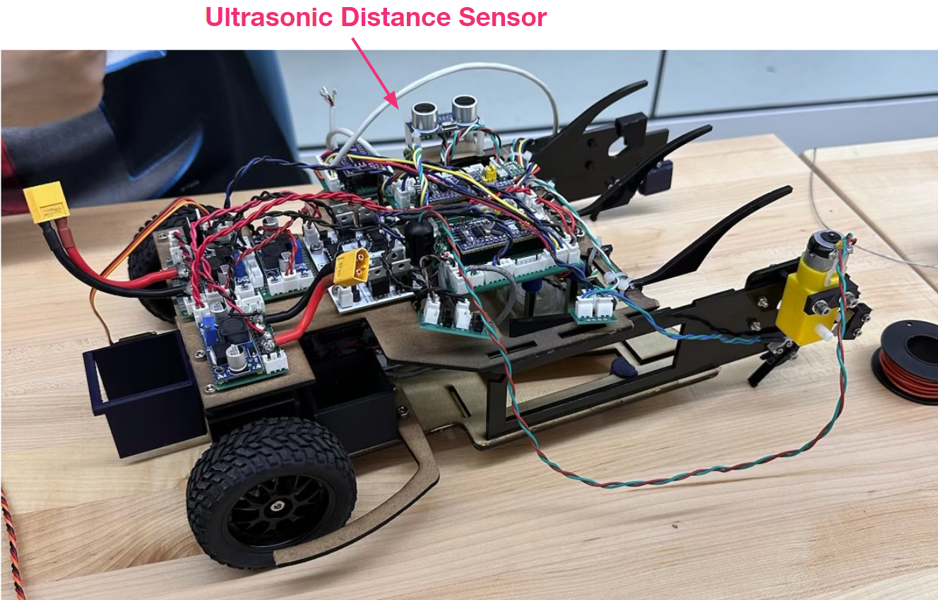
To understand our position on the track, we use sensors to look for identifiable physical track markers.
The first sensor we use is a HC-SR04 ultrasonic distance sensor to detect the bridge and the archway. The distance value appreciably changes when the robot …
- enters the bridge
- exits the bridge
- enters the small archway
- exits the small archway
We map these changes to states ENTERING_BRIDGE, BRIDGE, EXITING BRIDGE, PRE (for pre-archway), and POST (for post-archway)
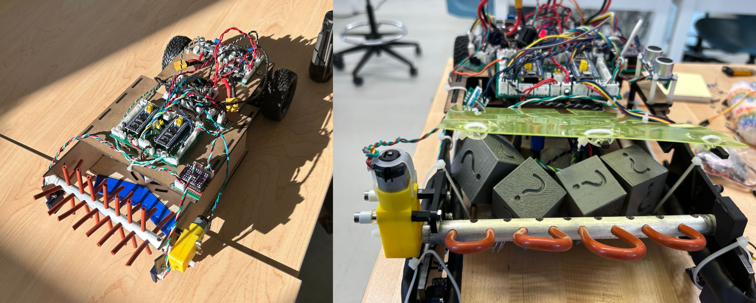
This sensor alone maps out the entire track from the start to right before the upwards ramp. But that leaves us to detect the up-ramp itself, rainbow road, and the down-ramp. To do so, I suggested we use physical switches located at the front of the robot:
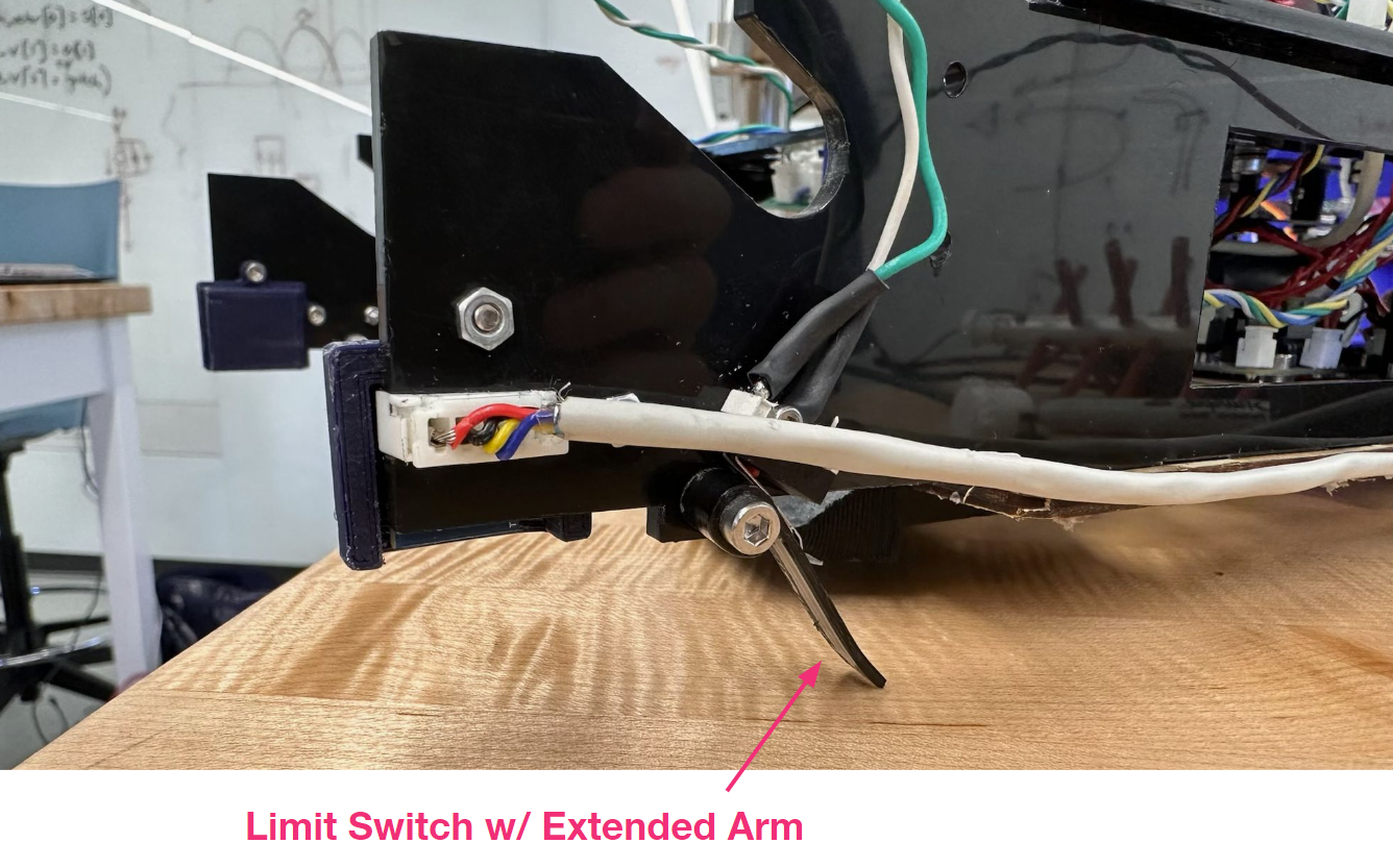
These are angled precisely and are slightly flexible so that they’re free to flap around and scrape along the surface of the track, but they physically click when the robot …
- starts going up when it reaches the upwards ramp
- starts going up rainbow road
- starts going down the rainbow road arch
- comes off the end of the downwards ramp
This clicking allows us to map the rest of the track into zones UP_RAMP, UP_RAINBOW, DOWN_RAINBOW, and TURN, which is the first state (since coming off the downwards ramp means we’re at START(2), which has a sharp turn.
And that gives us the final mapping of the track which I showed previously. The transition from TURN → START is simply handled by a timer, which ventures into the unfortunate region of hardcoding, but it’s what we had to do.
.png)
Note: Bomb Drop
Unfortunately, we didn’t save any videos of our bomb dropped in action, but we did use it throughout the competition. One benefit of using zones is that our robot can drop the bomb in 9 different spots on the track based on the team we’re competing against.
b) Bridge Handling
Implementing zones also helped solve one of our largest problems — the finish line. To us, the finish line is a nice indicator that a robot has fully completed a lap. But to the robot, the checkered black and white marks look like a complete mess, giving you an arbitrary error value. If you approached the line head on, you’d likely be able to cross the finish line just because you’re already aligned — but if you’re the slightest bit angled, you can be misled by the tape and ram into the side of the track:
.gif)
This is an issue that almost all teams faced at one point, but I’m not sure anybody fully solved. For us, the trivial solution would just be to slow down when we come under the bridge, so that we’re not wobbling as much and can align ourselves better. However, since the bridge (and the junction) is a big point of contention in the race, slowing down here is unfavorable and could possibly lead to collision.
Trevor had the interesting idea that, for when we’re under the bridge, perform PID with the error being the displacement off the middle of the archway. And this is not a bad idea in theory because regardless of what the tape sensors see, we can use the sonar to check the height of the bridge that we’re under, and then correct accordingly:
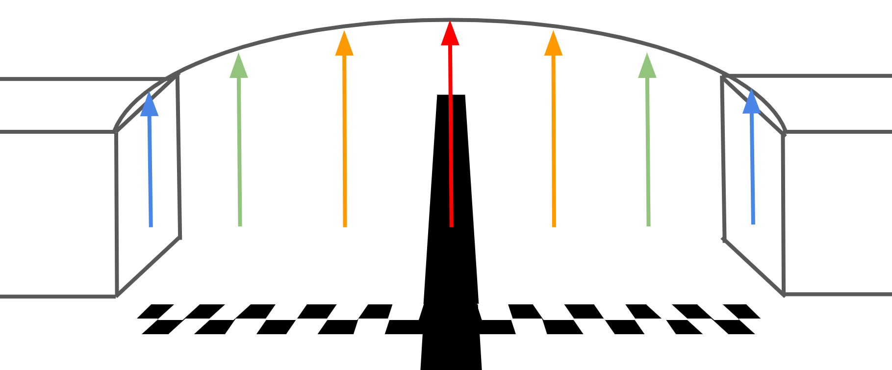
Unfortunately, this doesn’t work entirely because the archway is symmetrical, and so with one sensor, equal distances away from the line, whether it be left or right, will look identical to the distance sensor. This is shown by the same colored arrows, where two different positions under the bridge can alias into the same distance reading, so the PID won’t know whether to go left or to go right.
However, this got me thinking about using physical indicators on the track, and so I suggested we do the following:
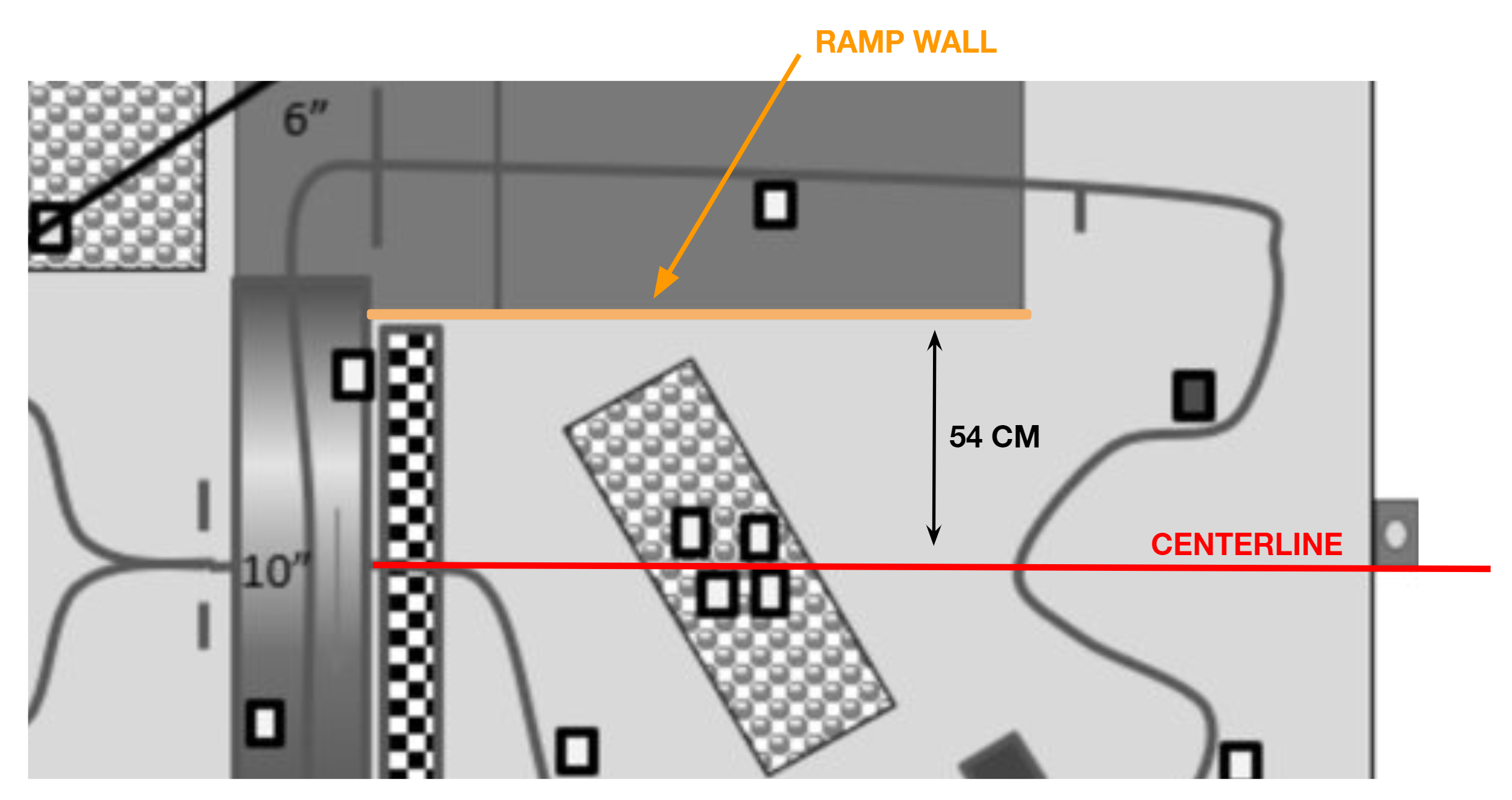
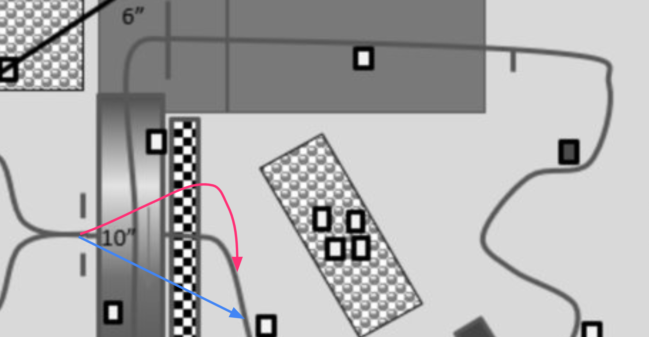
Here I’ve indicated the side wall of the ramp in orange, and the centerline in red, which are spaced ~54 cm apart on the track. If we’ve exited the bridge and we’re on the centerline, that means we weren’t misled by the tape. So how can we ensure we stay close to this line?
Simply place a distance sensor on the left side of the robot, so that as it exits the bridge, it reads the distance between it and the ramp wall. If that value is less than 54 cm, we’re too close to the wall (above the center line), so we need to shift right. Otherwise, if the value is greater than 54 cm, we’re too far away from the wall (below the center line), so we need to shift left. This way we can ignore the arbitrary error value from the tape track and overwrite it with the error .
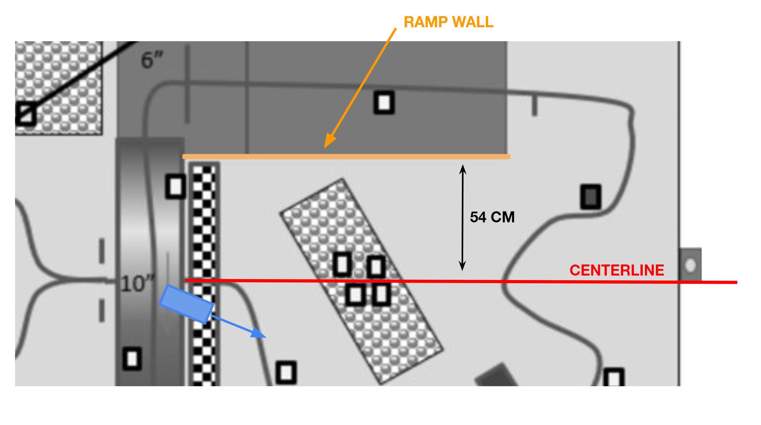
Here you can see an extreme case of that process in action, where we approach the finish line at a horrible angle, but the distance sensor reads that we’re too close to the left wall, and so it forces the robot to turn right.
.gif)
There is room for one more optimization though. If we’re exiting the bridge and we see that we’re too far away from the ramp wall, there’s no reason to shift left, because a little in front of you is the track anyways. So what we do is say that in this case, just keep driving forward until you hit the tape again:
This minor cut doesn’t look like much, but if we’re going to correct our orientation with respect to ramp wall when we exit the bridge, there’s no point doing any PID while we’re under the bridge, since we’ll be fixed by the time we leave it. So the final optimization we do is simply drive straight at full speed under the bridge. If we end up too close to the ramp, we shift right until we hit tape (shown in red), but if we end up too far away, we just keep going straight since we’re bound to hit tape in front:
The blue cut is a time save of about ~1s, and while it looks like the red path would add time, because we’re driving at a faster speed during this bridge region, we don’t end up losing any time at all.
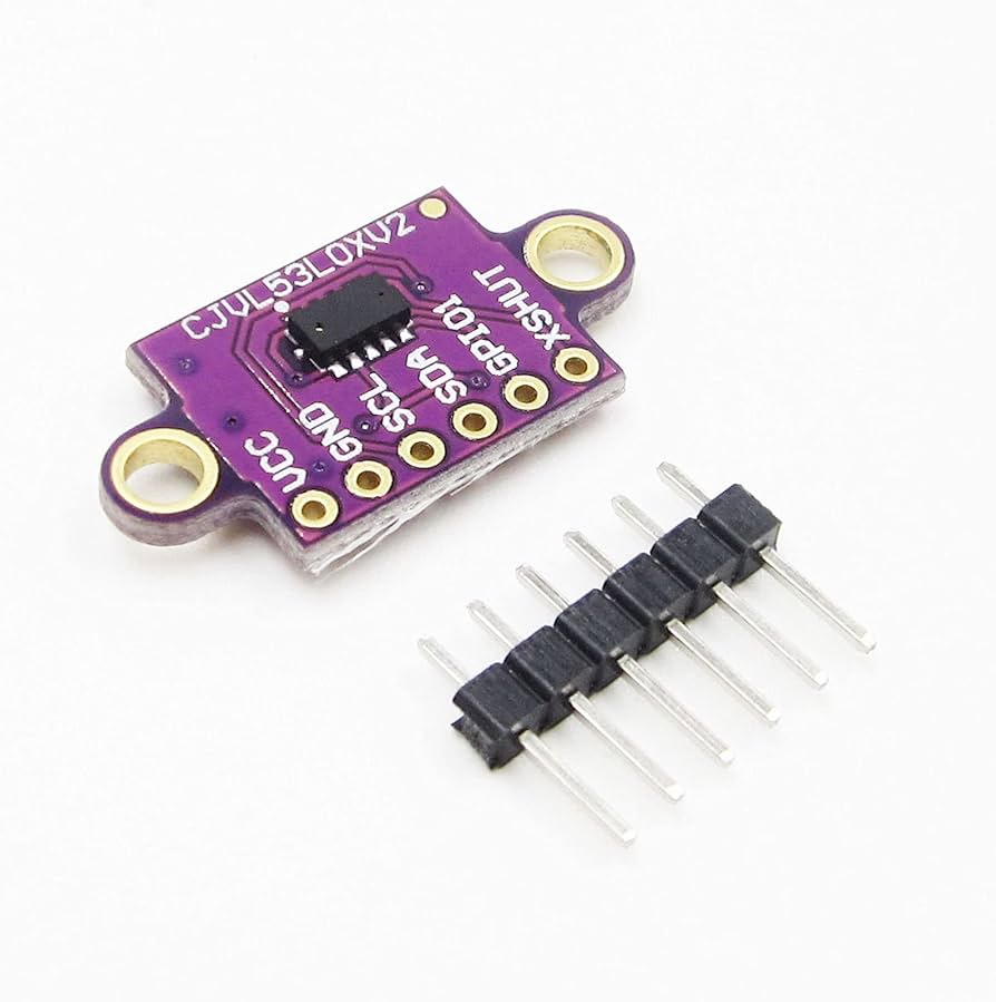
Note: VL53L0X Laser Distance Sensor
This scheme requires the distance reading between the ramp wall and the robot to be precise, so we use the VL53L0X laser distance sensor. It communicates over I2C and can give readings on the mm scale — it’s also very tiny which is why you can’t see it in any of the videos, but it’s mounted on the left side of the robot (the side which faces the ramp wall as the robot exits the bridge).
6. CAD + Run
Amr and Trevor did most of the CAD and machining throughout the course, but I was able to help them with some parts like the battery holders, motor shaft, side walls, and some other minor parts here and there. Since we went through lots of redesigns through the course, I pulled a few all-nighters with them so they could print / laser cut and assemble the parts in the morning.
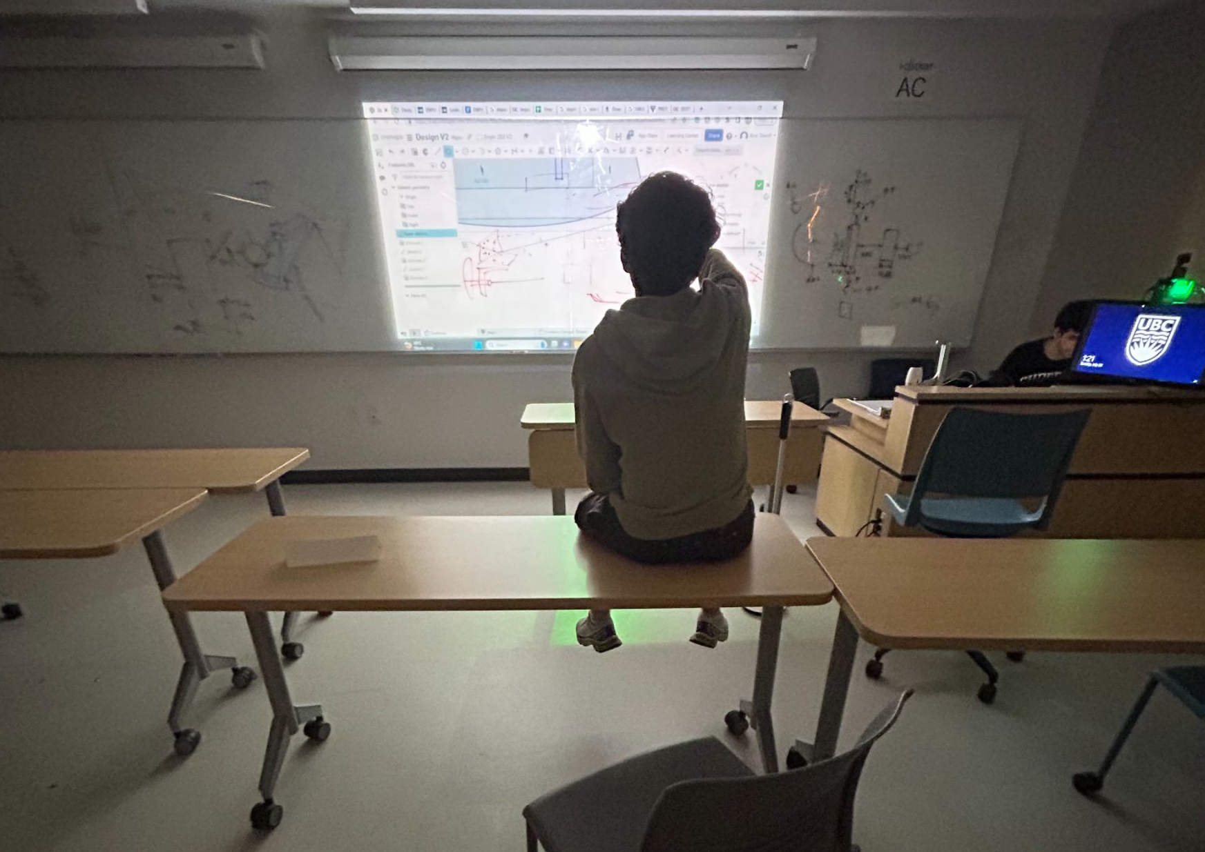
We projected the CAD window onto a whiteboard, and our workflow consisted of one of us actually designing it, and the other two labelling points on the whiteboard of what to adjust, cut, modify, or extrude. Here you can see Amr on his designing shift while Trevor and I tell him what to do 😅
And before I finish off here’s a demonstration of a ~16 second lap, without the shortcut being taken.
.gif)
I’m currently going through some of the live competition footage to see if I can find a clip of our full robot operation, where we’d drive around, pick up blocks, and drop bombs.
7. Conclusion
… and we’re at the end. I’ve been asked about my experience lots and about “how to win robot summer”. And of course, 2nd place isn’t a win, but here’s what I can say. And to any future ENPH 253 students who bothered to scroll this far, I would say this section is more important than anything I’ve written above.
The simple answer is that the competition changes every year, and then so does the strategy, which is extremely crucial for your success. That doesn’t mean there’s one way to win, it just means that you should choose something maintainable. If something seems overcomplicated while you’re planning, it will certainly get worse once you actually have to design, implement, test, and debug it. Problems will come up that you can’t even imagine.
“Does that mean I should choose the simplest strategy? Won’t I learn more if I try to do something complex?” No, and no. If you choose the easy way out, you can certainly do well, but you’ll end up learning almost nothing. If you try to do too much, the mere 6 weeks you have (and trust me, time flies) to build such a complicated robot will have you making poor design choices, rushing manufacturing, and being unable to test thoroughly. In fact I argue that you’ll learn even less than those who take the easy way out. So of course you should try something new, but if it gets too hard down the line, always be prepared to change up your plans and simplify.
Now, strategy and solutions are different. Within your appropriately-chosen strategy, you will come across various roadblocks in this course, and then I say the solution to those mini problems should be as simple as possible. When trying to detect the ramps, we wasted time with gyroscopes, level detectors, and even color sensing for rainbow road. But the simplest solution, and the most consistent one, was to just place some switches at the front and wait for them to click. ENPH 253 is about rapid design, and the longer you take on one thing will affect everything else you have to work on.
Then comes the engineering — it’s hard to perform well with an amazing strategy, but bad design. Don’t just build things that work, build things that will last. Try not to overcomplicate the software, keep your circuits clean, and build your robot in a way that’s easy to test, modify, and assemble. I can’t count how many times we assembled half the robot, only to realize we couldn’t tighten a nut because of how hard it was to reach.
But once you’ve done all that, it’s competition day. From what I’ve seen this year, and in talking to peers who competed in this competition anything above top 4 was unpredictable. If you ran the competition multiple times, those who get knocked out early would likely get knocked out again. But if the semi-finals were ran again, I can think of countless ways in which we get 3rd, 1st, or 4th. I went into ENPH 253 hungry to win, but I soon realize that everyone has brilliant ideas that never even crossed my mind. And especially when two vastly different robots race, if they both work consistently, it’s almost impossible to tell who will win.
In ENPH 253, I don’t think any robot was the “best”. If your robot has a theoretical statistic of 80 in pickup, and 20 in speed (80+20=100), you will almost always beat a team with 70 in pickup, and 10 in speed. But will you win against a team of 50 in pickup, and 50 in speed (50+50 is also 100)? And these are just two factors — in reality your robot has statistics in speed, block pickup, bomb avoidance, IR following, zipline mounting, jumping, collision detection, lap consistency, and more.
In my opinion, the best you can do is try a section of it all — think and work on speed, block pickup, bomb avoidance, IR following, zipline mounting, jumping, collision detection, lap consistency, and more. We didn’t do all of them, and neither did any other team. Those who did more on the list, weren’t as good as other teams who focused on a fewer handful. So who is better? In fact you’ll never really know, because it can come down to something that’s out of both team’s hands — like the placement of blocks, or the lighting in the competition room.
The only thing that you, and the rest of your peers will be able to agree on, is what you were able to accomplish. And boiling that down to a competition placement doesn’t tell the full story. In my year, a team that successfully travelled the zipline, but didn’t make it to top 4, received immense accolades from everyone and the program director himself. Another team that was knocked out early on still gained the respect of several in our year because they were able to complete a lap without following any tape. And the team that finished 4th had one of the nicest bomb avoidance mechanisms, intaking the bomb but then letting it slide out later.
The concept of anything but first can be pretty foreign to understand, and pre-robot-summer Ebrahim would have probably laughed reading this. But I’m proud that we figured out how to drive around within the first week of the course, and we didn’t stop there. We learned how to pick up blocks, map out the track, detect bombs with compasses, fix noise, put it all together, and make it work over and over again. I have an immense amount of respect for the teams that pushed the limits on what was possible within these 6 weeks. Even if something didn’t work all the time, they were able to show that at least it was possible.
And I truly believe that’s what ENPH 253 is about. It’s a course where you see new ideas come to life, not plain, boring ones. It’s about imagining something new and then actually going out and doing it. To those taking the course in the future, I hope you find such a course like this thrilling, push not to take the easy way out, learn a lot about yourself, and have fun all the way through.