FPGA FIR Development

In this documentation post we outline the development and usage of custom, runtime-adjustable FIR filters and their simulation on MATLAB, implemented on the Red Pitaya.

Background

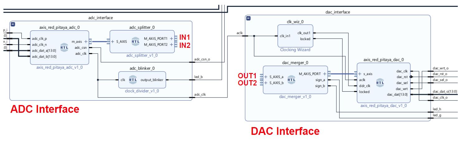
In the previous documentation bit, we made the individual ADC and DAC interfaces.

ADC:

The ADC interface translates the voltage on the input ports IN1, IN2 on the Red Pitaya to a 15-bit (1-bit MSB sign, 14-bit LSB data) data stream sampled at 125 MHz. IN1 data is provided on M_AXIS_PORT1, and IN2 on M_AXIS_PORT2.

DAC:

Inversely, the DAC interface translates a 15-bit signal (1-bit MSB sign, 14-bit LSB data) stream sampled at 125 MHz to an analog voltage. S_AXIS_a corresponds to OUT1, and S_AXIS_b on OUT2. The following image shows the ports to which we can access the analog/digital interfaces, and the corresponding physical headers they connect to on the Red Pitaya itself.

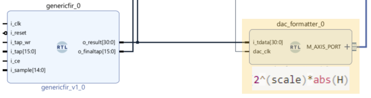
Details on this construction are available in the previous post. Any operation we want to implement will be placed within the purple placeholder box shown below:

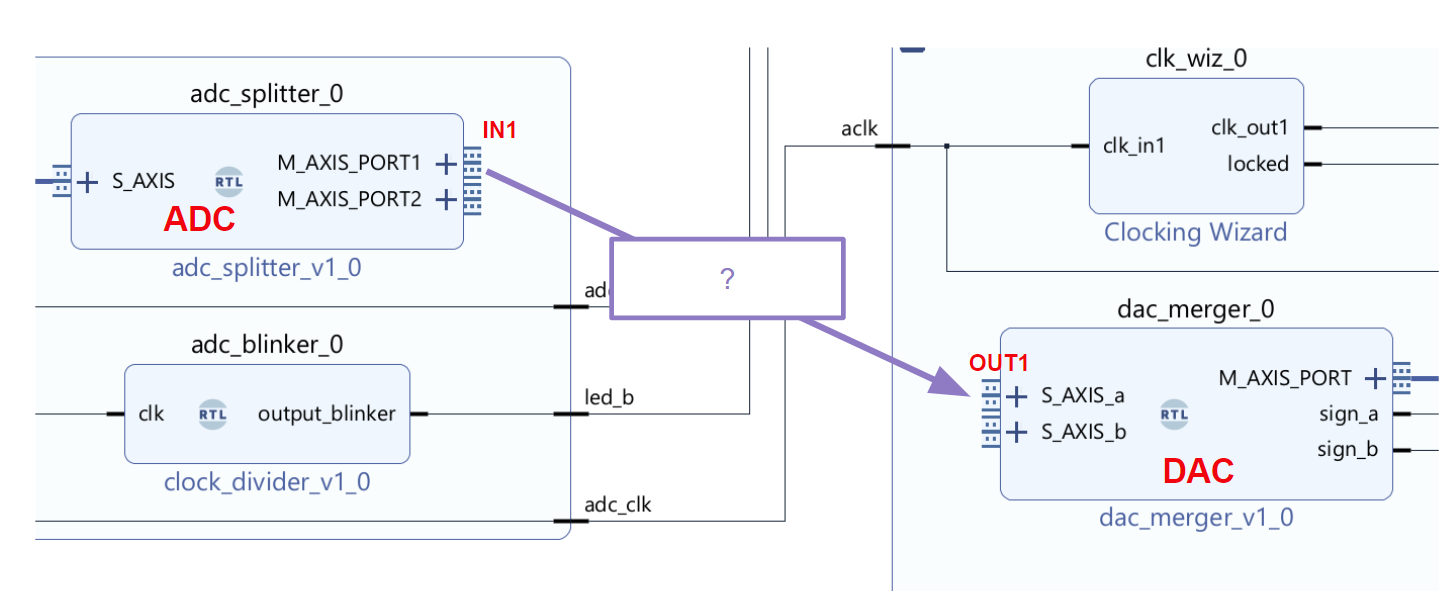
If no operation is placed, and we directly short the M_AXIS_PORT1 → S_AXIS_a data streams, the Red Pitaya will act as a glorified wire from IN1 to OUT1. Now, we will look into implementing an FIR filter within this operation box.

What to Avoid

Before we go into what we have created, first we discuss what we tried and why we avoid it going forward.

Xilinx provides their own FIR filter core for which we can enter in FIR coefficients (these coefficients determine the filter’s frequency response). However, it requires some extra cores to work on the Red Pitaya, as shown below:

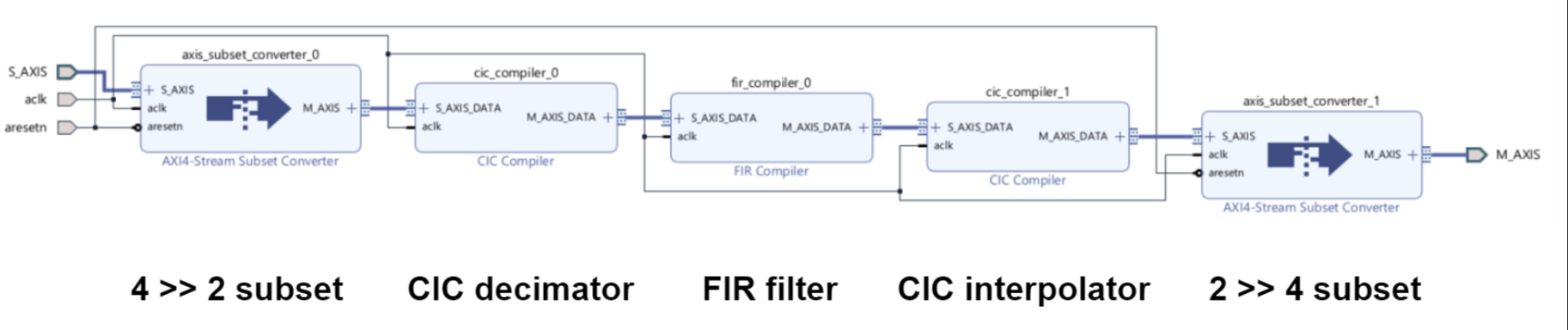
This entire system should in theory function as a hardware filter on the Red Pitaya. The FIR filter is encapsulated in the center, but after trying nearly everything, here are the best results we could get.

In this example we are trying to design an FIR filter with the following frequency response. We have already collected the coefficients, and are trying to plug them into the FIR.

Firstly, the surrounding CIC decimator and CIC interpolator have their own frequency response.

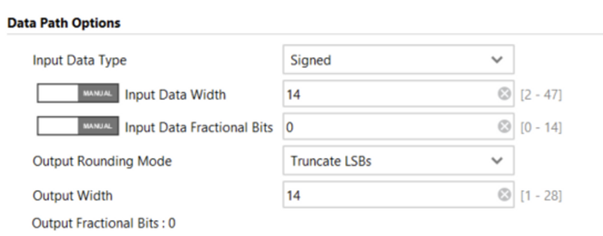
When we set the input data width of the FIR filter (14-wide, as it comes from the ADC), the FIR automatically suggests an output width of 52 bits .. this is unusable for two reasons:

• the CIC interpolator after the FIR can only handle a maximum of 32 bits as input

• no matter what we choose, the final data sent to the DAC must be 14 bits wide.

So, we have to select the output rounding mode as Truncate LSBs and forcibly round down within the FIR configurator:

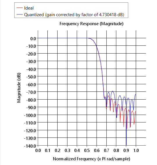
Placing in our coefficients, Xilinx reports the following frequency response. It suggests that when physically implemented, the gain will have to be corrected by 4dB.

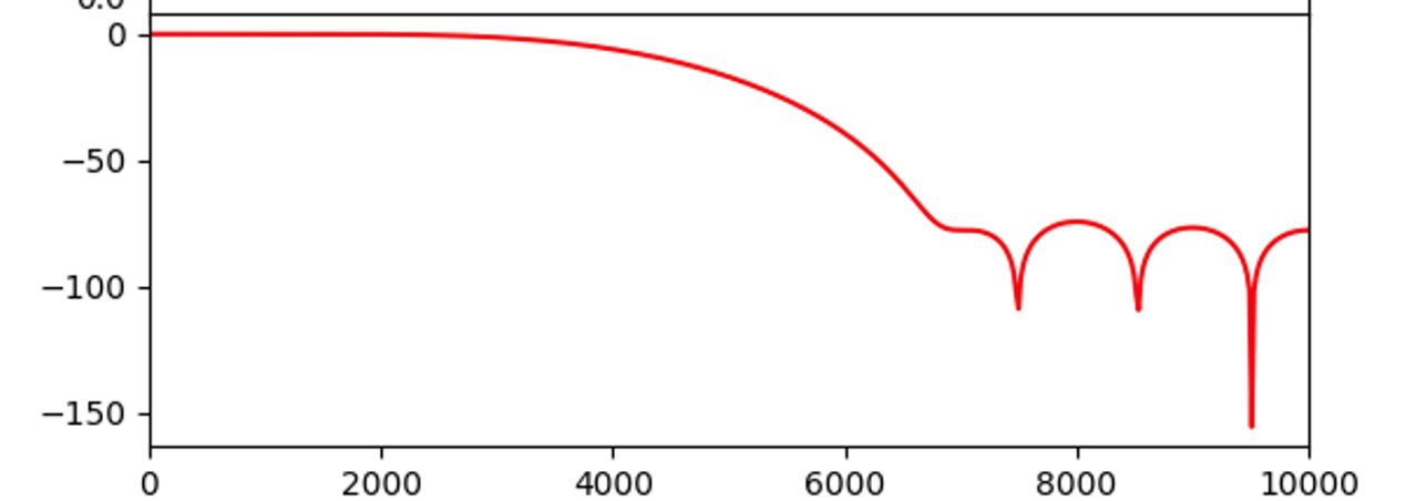
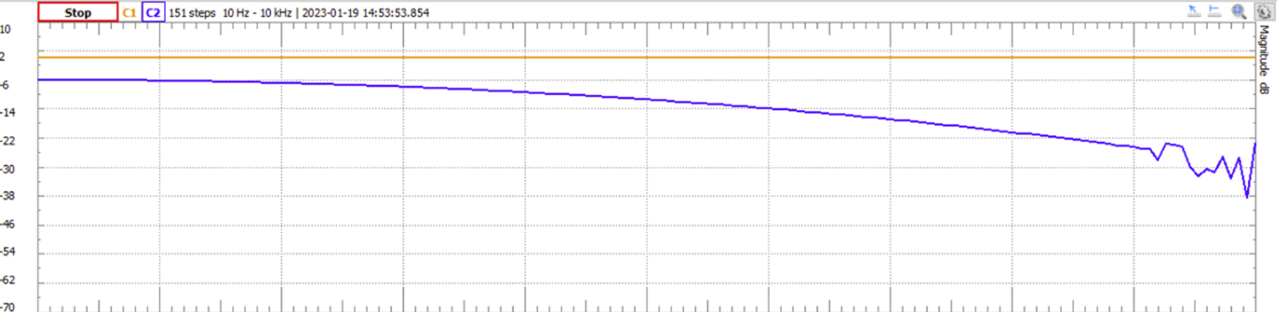
This results in the following overall frequency response of our filter setup:

Though the overall characteristic shape follows what we expect, the obvious issue is that the in the passband, the gain asymptotically reaches -10dB rather than the expected 0dB. The Xilinx FIR IP does NOT report this behavior and can only be obtained experimentally by a network analyzer. Xilinx’s reported gain is incorrect because we have a CIC filter before it. Again, two issues arise:

• it is rather abrasive, and the gain is now shrunken to <1 in the passband.

• we have no way of predicting how bad the rounding + gain adjustment will be due to the hidden code of the Xilinx FIR core.

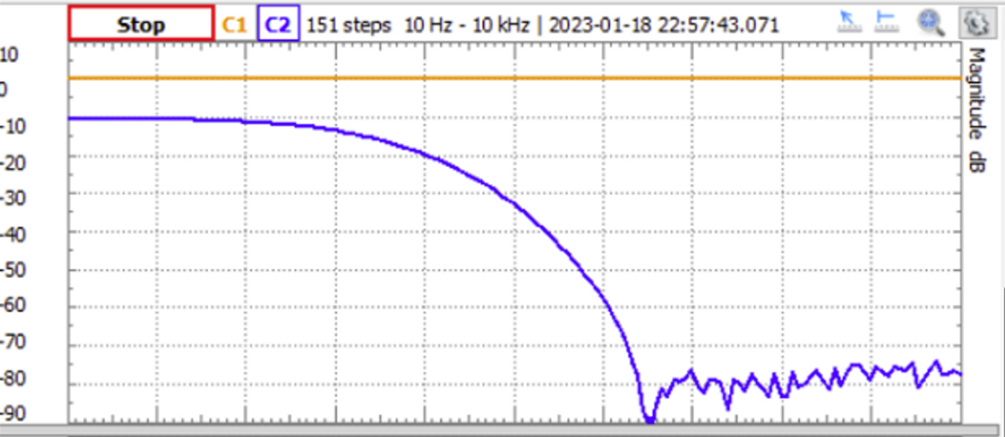
One workaround which does work is adding a rounding adjustment module, which essentially multiplies the FIR filter output by some constant $C$ such that in the passband, the maximum amplitude is at 0dB, such that we can obtain a curve like this:

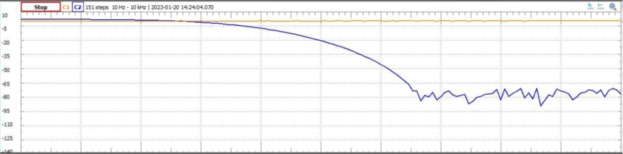
Now, the passband gain is ~0dB as required. So yes, maybe we do have a working FIR filter as of right now, but there is a lot of guesswork in finding this constant $C$ to get it working as intended.

What leaves us to eventually abandon this is the concern of flexibility. If we change the constants of the filter, we need to use the network analyzer again to find the discrepancy between the passband gain and 0dB, and then solve for the multiplier constant $C$. However, the end fact is that, if we use the FIR filter within a locking scheme, it will be enveloped by an array of other hardware. This makes it impossible to test the frequency response of it alone, and so it is impossible to solve for $C$ post-bitstream-generation without guessing.

Even then, hypothetically suppose the gain correction reported by Xilinx was correct:

Since it only appears in the editor, we have no way of accessing this value post-upload. So, if we ever change the coefficients, we will not know the new correction multiplier.

Our Implementation

Clearly the Xilinx core is too finicky and not built for runtime-adjustable changes.

After our meeting with Mandana we review and reclarify some design goals. Our final FIR filter should be able to:

1. function with reprogrammable coefficients during runtime (ie. we can change the frequency response at any point post-physical-implementation)

2. simulate its behaviour in MATLAB (or any external program) and observe the same experimental response (unlike what we experienced with the Xilinx core).

We outline how it is made and how to use it below.

Here is a 3-tap filter on our new FIR implementation:

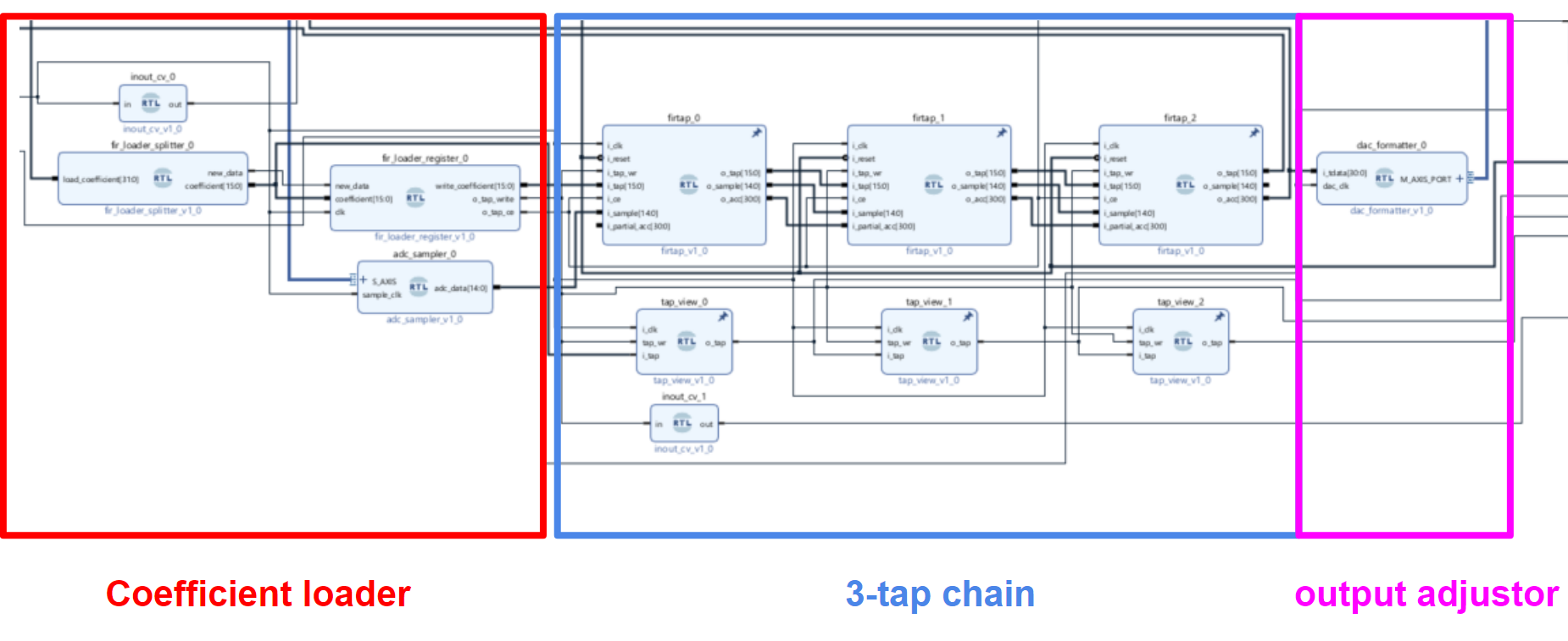
The modules are a little blurry, but we will zoom in further soon. There are three distinct partitions of this filter: the coefficient loader, the tap chain, and the output adjustor.

Coefficient Selection and Filter Simulation

Let’s step back a little and look at what we use to generate our FIR coefficients to begin with.

1. Make Full Precision Coefficients

The first step is to obtain a list of full precision coefficients, which is the set of FIR coefficients generated if we had theoretically infinite precision and perfect implementation. Since this step is isolated from the actual design of our FIR, we can obtain coefficient sets from websites like http://t-filter.engineerjs.com/, or MATLAB.

For lowpass filters, I had success using fdesign.lowpass (https://www.mathworks.com/help/dsp/ref/fdesign.html). The full precision coefficient list is c.

N = 19;                  %% number of taps -1     
Fsample = 100e3;         %% fir sampling frequency

Fpass = 25e3;
Apass = 0.05;
Astop = 50;
coeff_width = 16;
adc_width = 14;

% obtain quantized coefficients (cq)
designSpec = fdesign.lowpass('N,Fp,Ap,Ast', N, Fpass, Apass, Astop, Fsample);
LPF = design(designSpec,'equiripple',SystemObject = true);
fvtool(LPF);
c = coeffs(LPF).Numerator;

For highpass and bandpass filters, I was able to use designfilt (https://www.mathworks.com/help/signal/ref/digitalfilter.html)

fs = 100e3;          %% fir sampling frequency
N = 30;              %% number of taps -1
coeff_width = 16;
adc_width = 14;

d = designfilt('bandpassfir', ...
    'FilterOrder',N, ...
    'StopbandFrequency1',10e3, ...
    'PassbandFrequency1',15e3, ...
    'PassbandFrequency2',20e3, ...
    'StopbandFrequency2',25e3, ...
    'SampleRate',fs);
fvtool(d)
freqz(d)
c = d.Coefficients;

Overall, designfilt seemed a little less finicky to use, but again we have considerable freedom in how we choose to obtain our coefficients.

2. Quantize Full Precision Coefficients

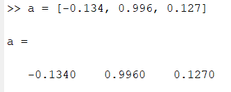
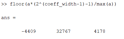
Of course, we are not creating an infinitely precise FIR filter on an FPGA. c will be a set of floating point numbers (eg. [-0.134, 0.995, -0.127]), but it is difficult to store these numbers on digital hardware. With our full-precision set c, we will now quantize the coefficients, which will turn them into integers, by the following formula:

cq = floor(c*(2^(coeff_width-1)-1)/max(c));     % quantized coefficients

Notice that this formula takes in the width in bits that we have to store our coefficients — for our purposes, we will use 16-bit coefficients. This formula simply linearly scales all floating point values (-1, 1) to integers on the range $(-2^{15},2^{15})$. Keep in mind that we perform coeff_width-1 since one bit is used to hold the sign of the coefficient.

3. Simulate Filter

With these FPGA implementation-specific coefficients, we simulate our filter using MATLAB. To do this, we pass our quantized coefficient list cq to a digital FIR filter simulator (dffir), and plot the frequency response. For our implementation, coeff_width is 16 (what we used to generate cq), and the Red Pitaya ADC data width is 14 bits wide (15 bit wide for sign).

fir = dfilt.dffir(cq); % <- pass cq we made earlier
fir.Arithmetic = 'fixed';
fir.CoeffWordLength = coeff_width; % 16
fir.InputWordLength = adc_width;   % 14
fir.InputFracLength = 0;
ss = fir.Numerator;
regexprep(num2str(ss),'\s+',' ') % print out quantized coefficient list
fvtool(fir, 'Color', 'white')    % plot frequency response

Suppose cq is the coefficient set generated by fdesign.lowpass (two code blocks above). The first plot we see is the frequency response of the FIR on its own:

At first glance, the general shape of the filter curve is right - we specified a cutoff frequency at 25kHz ($f_s/2$ = 50kHz), and indeed the amplitude drops at 25/50 = 0.5. However we notice that the frequency amplitude in the passband is 90dB, which is extremely high.

This happens because our quantized coefficients were all multiplied by a factor of at minimum $2^{15}$. Since the frequency response amplitude of the FIR is a discrete convolution:

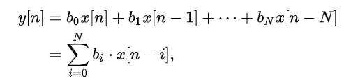
The output y[n] is multiplied by $\approx 2^{15}$. However, this is fine - we can scale the output result of the convolution as we wish until the maximum amplitude in the passband is 0dB (gain = 1). This is done with the following script:

scale = -coeff_width;
[H,w] = freqz(fir);                        % characterize the amplified response
tiledlayout(2,1);
nexttile
plot(w/pi, 20*log10(2^(scale)*abs(H)));    % scaled-down magnitude response (db)
nexttile
plot(w/pi, 2^(scale)*abs(H));              % scaled-down magnitude response (gain)
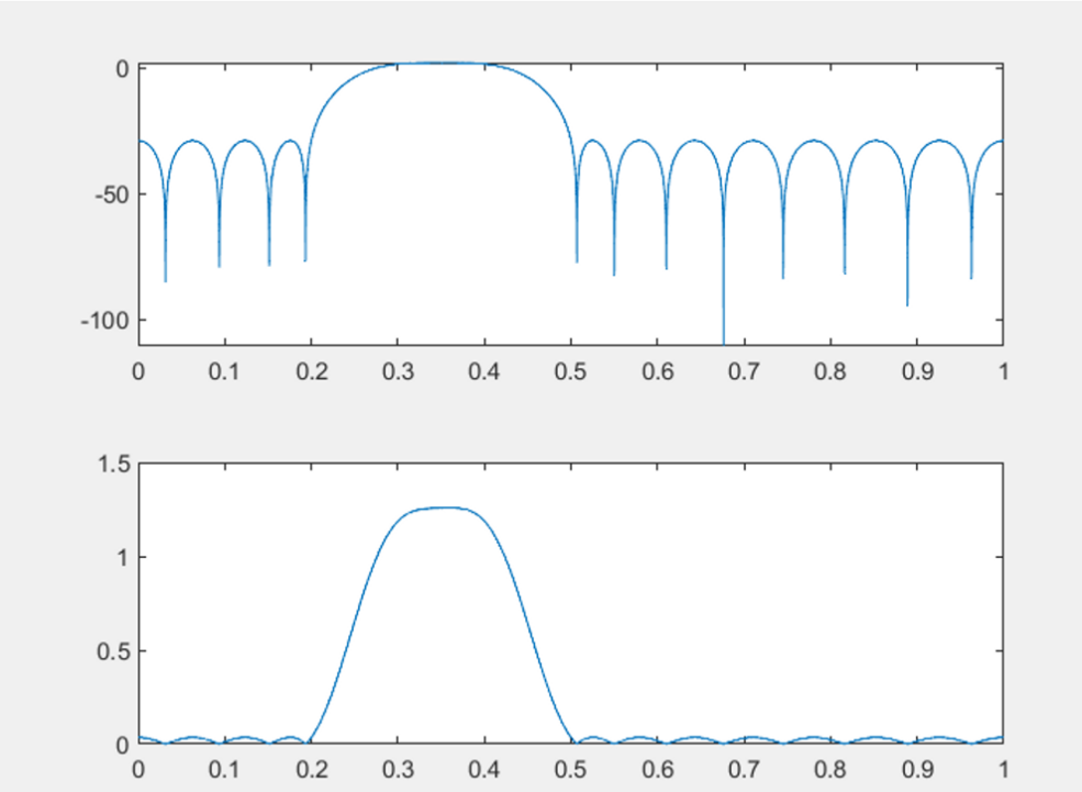
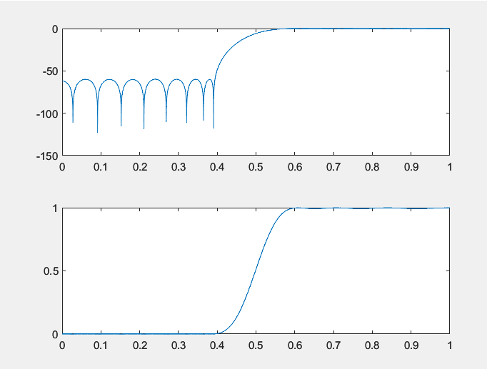
info(fir)

The scale coefficient will be close to or equal coeff_width to approach 0dB in the passband. Of course, there may not exist an integer for scale which sets the passband amplitude exactly to 0dB, but we can get reasonably close. Returning to our example, setting the scale to be -coeff_width, the output product is multiplied by $2^{-16}$ and is plotted below by our program (top dB, bottom gain):

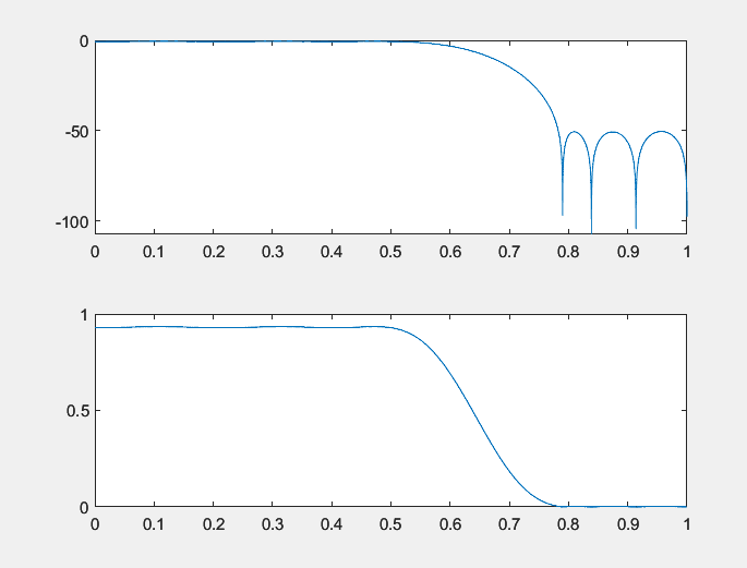
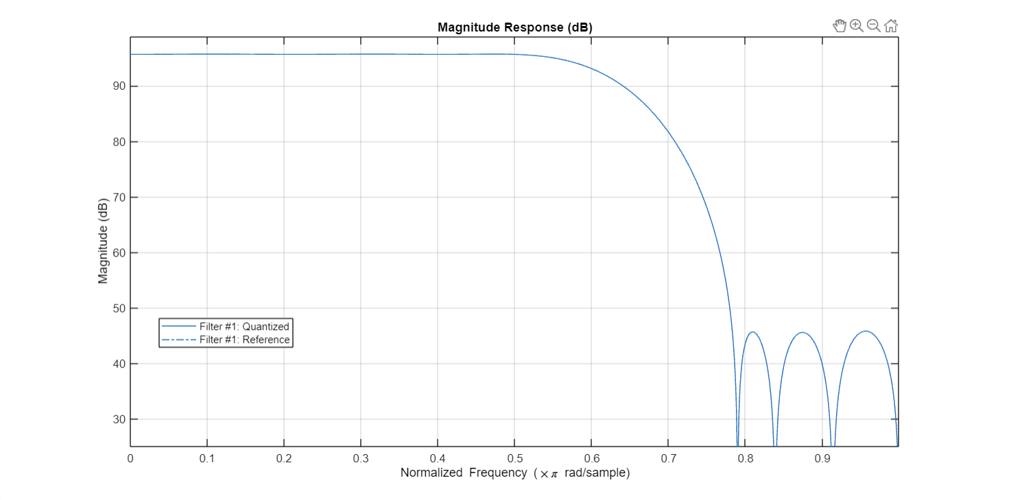
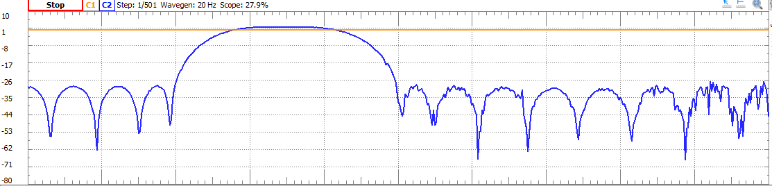
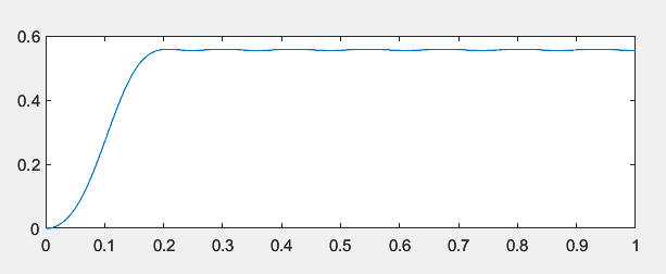
This is, for now, satisfactory. Ideally we would like to multiply the output product by an exponent of 2 so that in hardware, it can be represented by a bit shift. Let’s jump to the end for a quick moment and view the output result of the FIR filter with our quantized coefficients and output scaling:

Much better! Comparing with the theoretical gain curve above, we’re seeing extremely similar results.

What’s important here is not that the max amplitude response is at 0dB, but that whatever we simulate in MATLAB will be directly present on our hardware as well. This means that, if we desperately required a passband gain of 0dB, we can throw in another multiplier after the bit shifter to adjust as necessary.

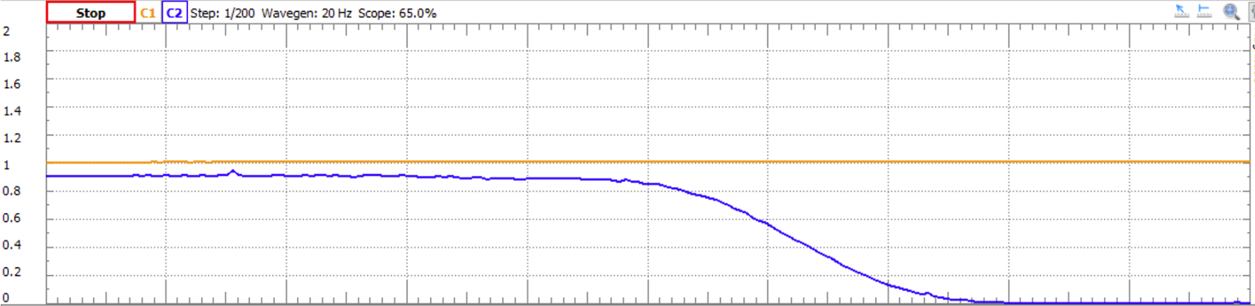
Just for fun, I’ll jump ahead again and show another example on the completed filter.. almost identical responses!

Hopefully now I’ve instilled some trust that we have a MATLAB simulator to accurately generate coefficients and plot the frequency response for a Red-Pitaya specific FIR filter. As discussed above, any more precise tuning we want to do such as adding a multiplier can be added on top of the MATLAB simulation as well. Overall, when we change coefficients on the fly in our final system, we have a guarantee that any transfer function we specify will be modelled exactly in hardware.

Coefficient Loader

We have just built a scheme to develop quantized coefficients - the next step is to send these to the FIR.

On a 20-tap filter with 16 bit coefficients, we would require a $20 \times 16 = 320$ bit input channel to write to all these coefficients at once (which will be stored within 320 registers). A smarter and expandable solution is by cascading tap coefficients through one input channel, as shown below:

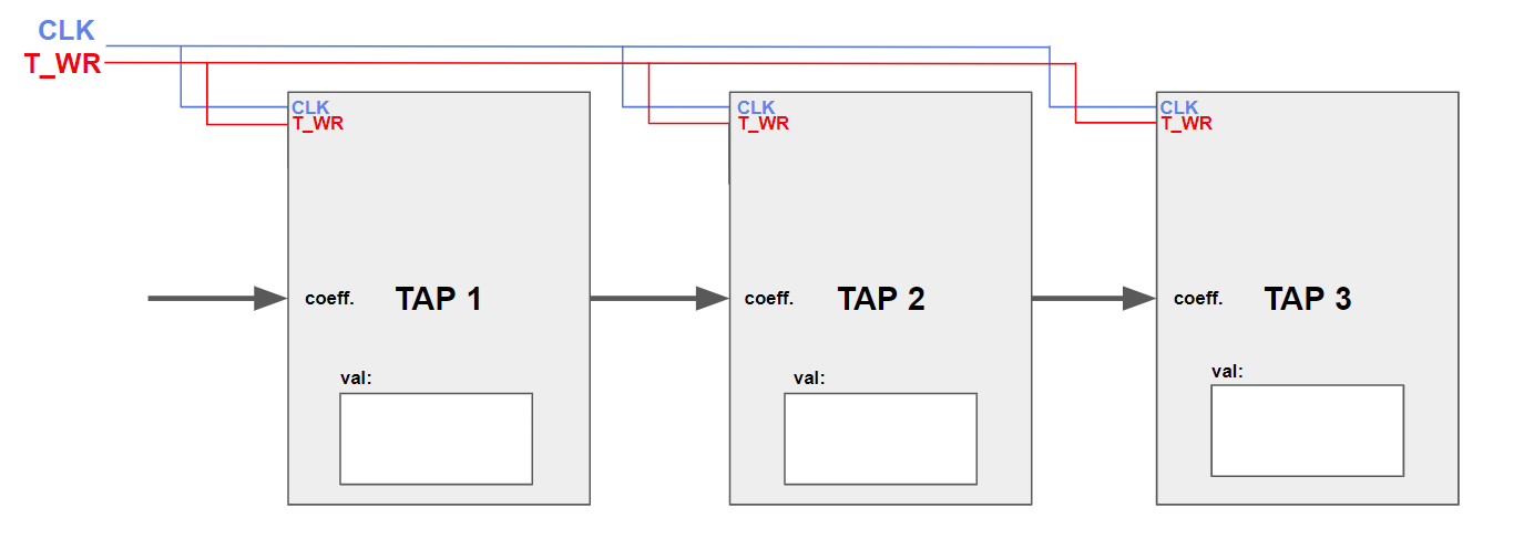
For our N-tap FIR (here, 3), we create a cascading coefficient line. We also establish a tap write signal T_WR. If T_WR is pulled high, tap coefficients will shift down the line on every rising clock edge (CLK).

Here is an example of how we would feed the coefficients “1, 2, 3” into the system:

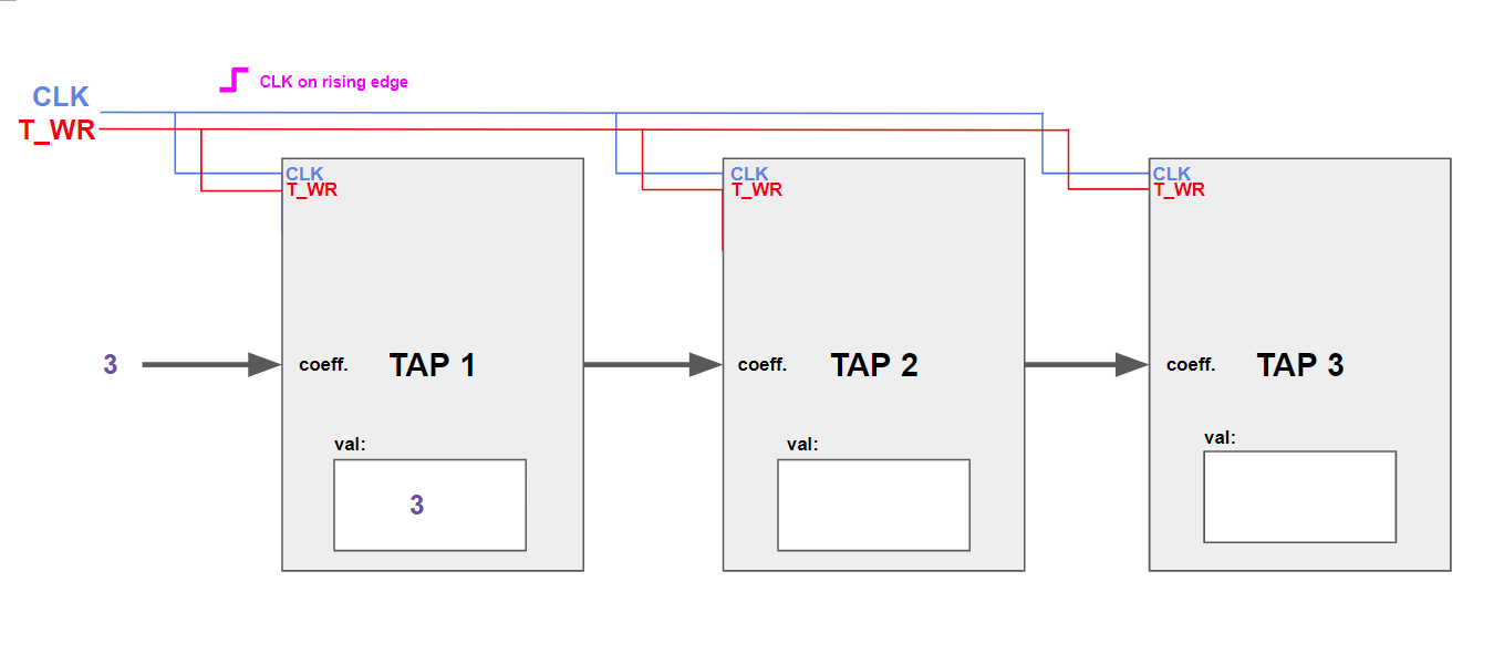
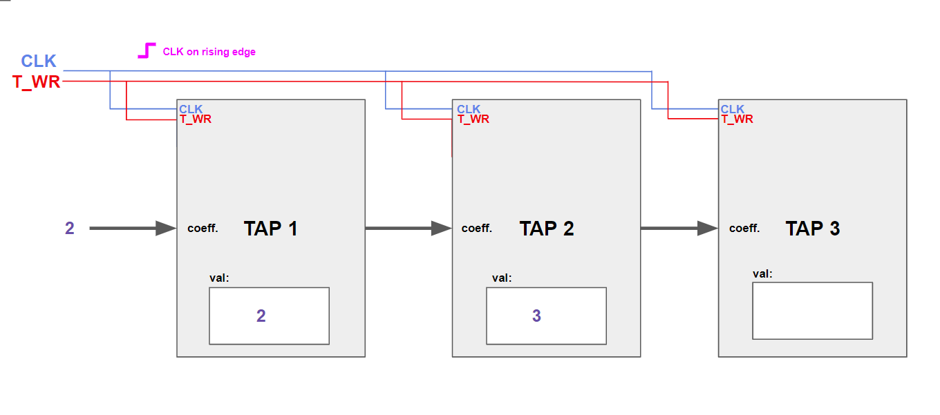
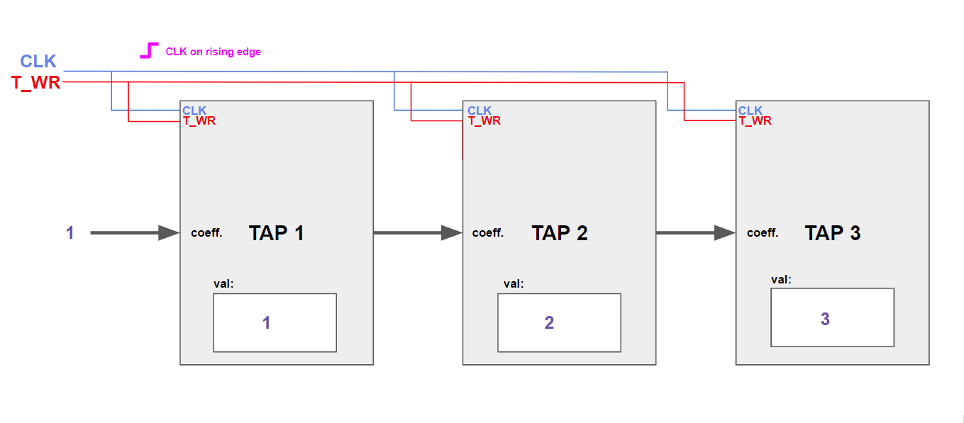
On every clock rising edge when T_WR is high, the value present on the [n-1]’th input is fed into the [n]’th register. This is a shift register! Notice that we have to set the data line to “3, 2, 1” in reverse such that the first number we send is shifted to the end of the line first.

This logic is present within each tap to enable this:

reg	[(TW-1):0]	tap;           // <- this holds the tap value in a register
initial	tap = INITIAL_VALUE;
always @(posedge i_clk)
if (i_tap_wr)                  // <- if tap_wr is enabled ...
	tap <= i_tap;                //    ... update thecurrent tap 
assign o_tap = tap;            // set output to current to shift prev. data

And here is a closer view of the tap structure in Vivado:

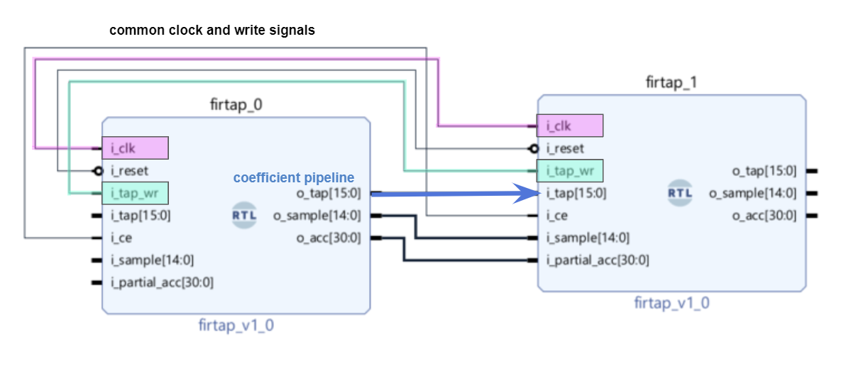
Our input coefficient stream (from the Linux side) feeds into firtap_0's i_tap[15:0], and we set tap_wr high for one clock pulse when we want to shift in a new coefficient.

To automate this process, we build a fir_loader_register which sits behind the first tap, and toggles the tap_write signal when a new coefficient comes into it.

module fir_loader_register(
// new_data = GPIO[16]      (17th bit)
    input  wire            new_data,   
// coefficient = GPIO[15:0] (0-16th bits)             
    input  wire  [15:0]    coefficient,             
    input  wire            clk,
    output wire [15:0]     write_coefficient,
    output                 o_tap_write,
    output                 o_tap_ce
    );
    reg new_data_delay;
    wire data_pulse;
    always @ (posedge clk) begin
        new_data_delay <= new_data;
    end
    assign data_pulse = new_data && ~new_data_delay;
    
    assign o_tap_write = data_pulse;
    assign o_tap_ce = ~data_pulse;
    assign write_coefficient = coefficient;
endmodule

The details for this scheme are 1) tedious to explain and 2) will likely change as coefficients will, in the future be loaded from RAM than from the Linux$\iff$FPGA pipeline as we do in this post.

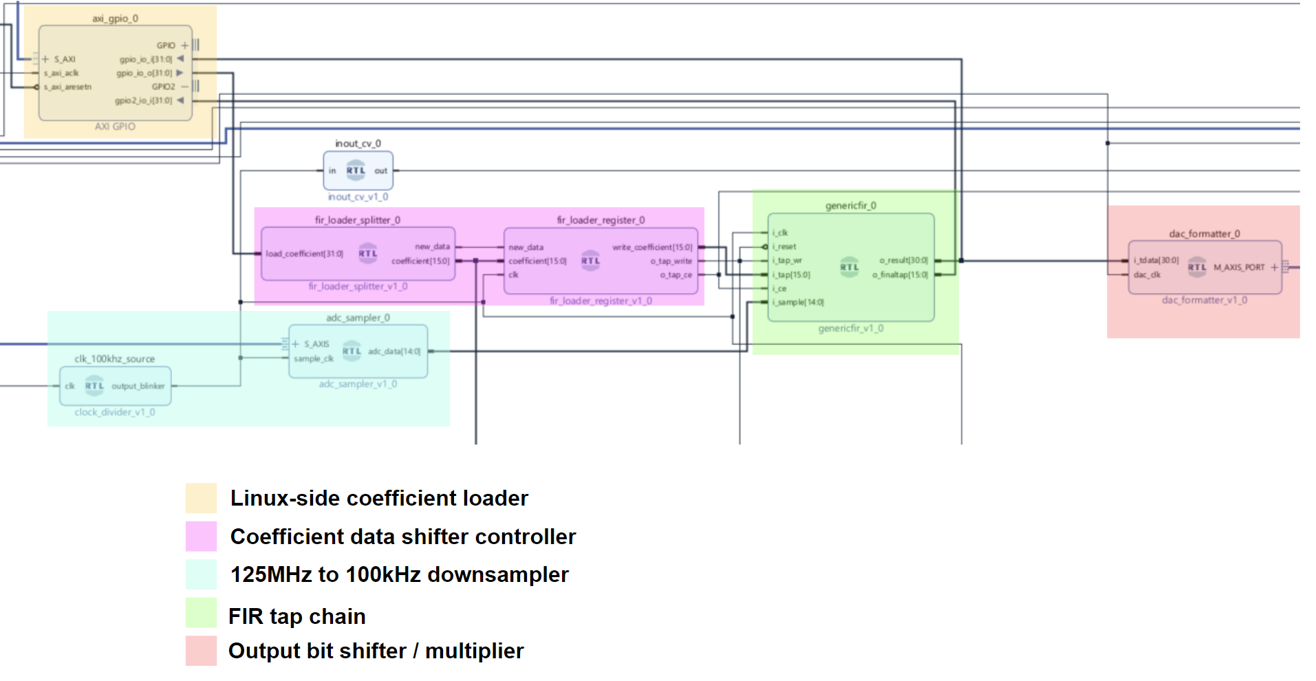
Here is the final construction:

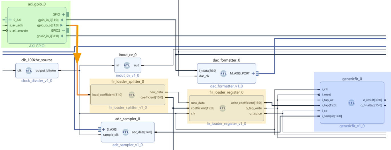
Coefficients come in from the Linux side (accessed remotely) through the axi_gpio block (green). It is split into a new_data and coefficient stream by the fir_splitter, which is sent to the fir_loader (yellow). Any time a new coefficient comes in by Linux, it is shifted into the tap chain located within generic_fir0 (blue).

For a N-tap FIR filter, we can shift in an entire set of FIR coefficients with the following code:

# coeff.py
from operator import*
import sys
import os
wr="10000"
coeffs = sys.argv[1:]                                 # remove the first element (name)
coeffs.reverse()                                      # reverse the list for shifting
print(len(coeffs))
for i in coeffs:
    os.system("monitor 0x41200000 0x0")               # send 0 to prepare for new data
    hexnum = hex(i & 0xffff)                         
    coeff = str(hex(add(int(wr,16),int(hexnum,16))))
	  os.system("monitor 0x41200000 "+coeff)            # send the hexadecimal coefficient

Coefficients are typed in order after the file name, with spaces in between as such:

>> python3 coeff.py 12309 34806 89735 ... 45627

With this script, we now have a way to reconfigure our FIR filter to act as a lowpass, bandpass, highpass, etc. type filter as we need.

Tap Arrangement

We use https://zipcpu.com/dsp/2017/09/15/fastfir.html (Building a high speed Finite Impulse Response …) and the associated GitHub: https://github.com/ZipCPU/dspfilters/tree/master/rtl (firtap.v, genericfir.v).

Our Red-Pitaya specific versions of firtap.v and genericfir.v are on Gitea (~/rtl).

To chain the taps together, we use a generate statement in Verilog to describe the structure — upon synthesis and bitstream generation, Vivado will compile that statement into logic.

Here is our modified version of genericfir.v, taking into account the tap shifting process.

module	genericfir #(
		// {{{
		parameter		NTAPS=3, IW=15, TW=16, OW=31,
		parameter [0:0]		FIXED_TAPS=0
		// }}}
	) (
		// {{{
		input	wire			i_clk, i_reset,
		input	wire			i_tap_wr,	// Ignored if FIXED_TAPS
		input	wire	[(TW-1):0]	i_tap,		// Ignored if FIXED_TAPS
		input	wire			i_ce,
		input	wire	[(IW-1):0]	i_sample,
		output	wire	[(OW-1):0]	o_result,
		output  wire    [(TW-1):0]  o_finaltap
	);
	wire	[(TW-1):0] tap		[NTAPS:0];
	wire	[(IW-1):0] sample	[NTAPS:0];
	wire	[(OW-1):0] result	[NTAPS:0];
	wire		tap_wr;
	genvar	k;

	// set inputs:
	assign	sample[0]	= i_sample;   // set signal input to first sample tap
	assign	result[0]	= 0;          // set initial sum input to 0
	assign tap[0] = i_tap;            // set coefficient input to first tap register
	

	// create tap chain
	// {{{
	generate
        // }}}
        for(k=0; k<NTAPS; k=k+1) begin: FILTERTAP
            firtap #(
                // {{{
                .FIXED_TAPS(FIXED_TAPS),
                .IW(IW), .OW(OW), .TW(TW),
                .INITIAL_VALUE(0)
                // }}}
            ) tapk(
                // {{{
                i_clk, i_reset,
                // Tap update circuitry
                i_tap_wr, tap[k], tap[k+1],
                // Sample delay line
                i_ce, sample[k], sample[k+1],
                // The output accumulator
                result[k], result[k+1]
                // }}}
            );
        end 
	endgenerate

    // output products:
	assign	o_result = result[NTAPS];
	assign  o_finaltap = tap[NTAPS];

endmodule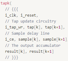

This section itself describes the cascading of the filter taps - clk, reset, wr, and ce are global, while the tap, sample, and result accumulations are shifted down each tap from start to end.

Output Adjustment

Finally, we perform the $2^{-\mathrm{scale}}$ multiplication post-FIR-output to bring the amplitude response down - this is what we simulated in MATLAB earlier! It sits right between the FIR output and the DAC’s data input. Shown in yellow is the operation it performs:

Here is the code, and since we’re multiplying by an exponent of 2, there’s no multiplication but rather we bit shift the data. Here’s a good place we could situate an extra multiplier should we need it in future tuning.

module dac_formatter #
(
    parameter ADC_DATA_WIDTH = 14,
    parameter AXIS_TDATA_WIDTH = 32,
    parameter FIR_DATA_WIDTH = 31,
    parameter SCALE = 16 // stored as 16, but shifts to 2^{-16}
)
(
    input  wire [FIR_DATA_WIDTH-1:0]        i_tdata,
    input  wire                             dac_clk,
    (* X_INTERFACE_PARAMETER = "FREQ_HZ 125000000" *)
    output wire [AXIS_TDATA_WIDTH-1:0]      M_AXIS_PORT_tdata,
    output wire                             M_AXIS_PORT_tvalid

);
    wire [ADC_DATA_WIDTH-1:0] data_reg;
    wire                      sign;
    
    assign sign = i_tdata[FIR_DATA_WIDTH-1];
    assign data_reg = i_tdata[SHIFT+ADC_DATA_WIDTH-1:SHIFT];
    
    assign M_AXIS_PORT_tdata = {{(18){sign}},data_reg};
    assign M_AXIS_PORT_tvalid = 1;
endmodule

Final Operation

We are finally done… here is a top-down view of the entire filter. The down-sampler / decimator is simply to slow down the sampling rate for the FIR.

Bandpass

MATLAB:

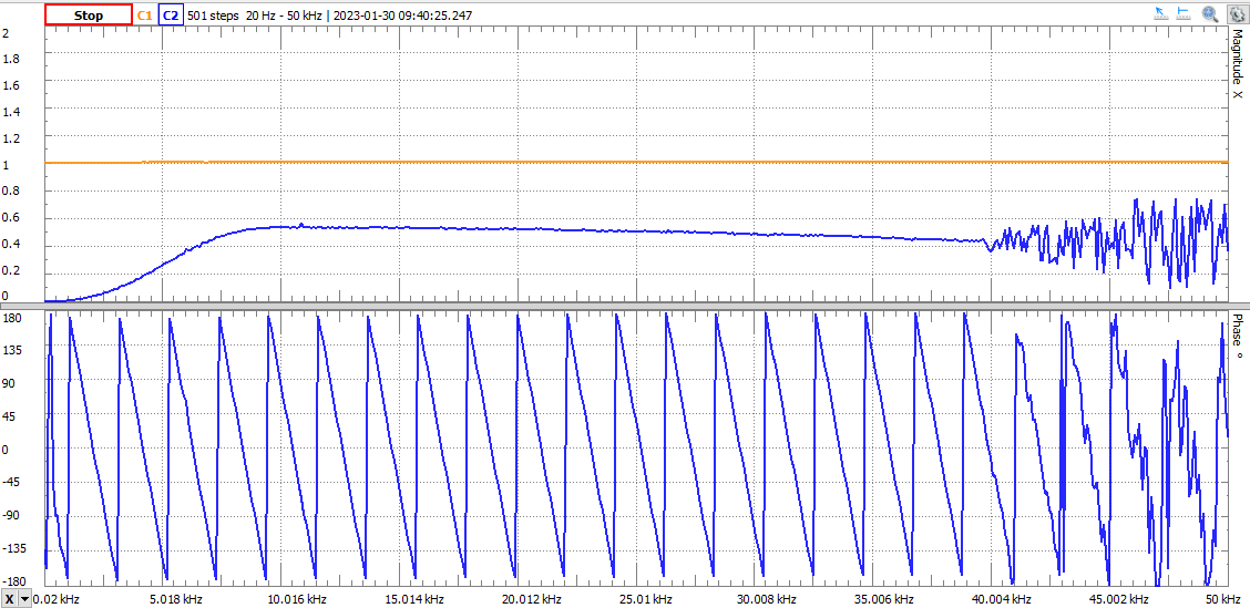
Experimental:

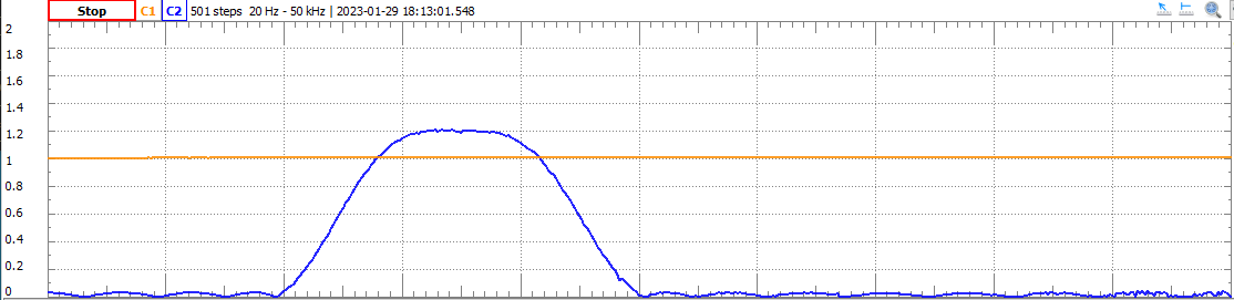
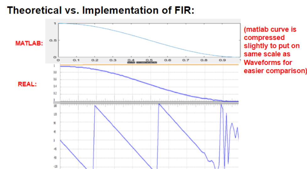
Highpass (2 attempts)

MATLAB 1:

REAL 1:

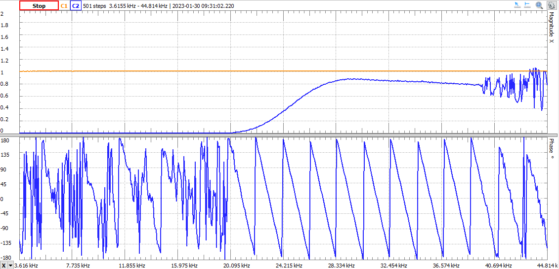
MATLAB 2:

REAL 2:

Our works well with linear phase for the majority of the pass/stop bands, so nothing is wrong with the filter programming or implementation. This issue lies further within digital signal processing itself.

Remember, we are down-sampling our input rate for the FIR filter - here is an exaggerated effect showing the effects of this decimation as frequency increases:

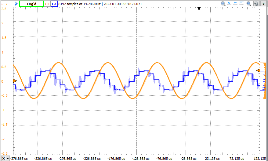
This works well across small normalized frequencies (0-0.5), but as we get closer and closer to $\frac{f_s}{2}$ (0.7 → 0.9), the decimated stream becomes either unreadable or too inaccurate:

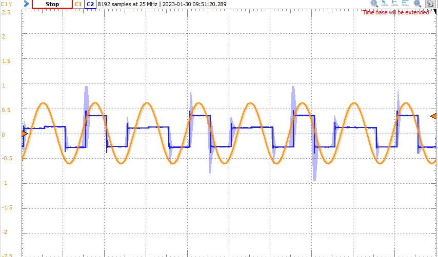
To solve this, if we want to develop a high-pass filter on the range of 0-50kHz, instead of setting the sampling rate to 100kHz (done above), we set it to upwards of 200kHz, such that the normalized peak operation frequency (originally 1) is now reduced to at max 0.5. Since we are using the Red Pitaya which samples at 125MHz and only need to use a couple filters, this is a change we can make rather freely without it being too costly in terms of LUT/DSP usage.

Final

We have developed a general purpose digital FIR filter that :

• is simulated and adjustable on MATLAB

• features runtime-adjustable coefficients to change filter type (lowpass, bandpass, etc.)

• can be placed in and around other modules (mixers, PID’s) without requiring individual tuning (unlike the Xilinx IP core)

• stable and precise with theoretical implementations up to normalized frequencies within $\approx$(0,0.7) (relative to $f_s/2$) … and like we said above, if we need to operate in the (0.7,1) range relative to $f_s/2$ , simply increase $f_s$ .

Should we need the FIR in a very precise application later on in the project, we should look at our own interpolation scheme as well, which can be placed after the dac_formatter.