FPGA CIC Development

As described here, if we decimate a signal to a new sampling frequency, the higher frequencies will alias into lower ones, adding noise into the signal. This aliased noise is greatly reduced by a CIC down-sampling filter.

The FPGA (Red Pitaya) samples at 125 MHz. But it’s requires a lot of resources to design a effective digital filter across the entire 0 → 62.5MHz (Nyquist frequency = maximum bandwidth = $\frac{f_\text{sampling}}{2}$) range. Say the signals I am interested in only working with have a maximum bandwidth of 1 MHz (1000 kHz). If that’s the case (which it very commonly is), there’s no reason to design a filter for such a large bandwidth. What we can do is down-sample the signal as much as possible before it reaches our filter, so that our filter only has to operate on the 0 → 1 MHz range instead.

So let’s try that! We can try is just decimation rate of about R=60 (order=1), so that we sample at $\frac{125}{60} \approx$ 2.083 MHz. Then the Nyquist frequency, which is the maximum filter bandwidth is $\approx$1.042 MHz. That’s just above the maximum signal bandwidth of 1 MHz, so we’re in the clear. We plug in important variables into the cic_designer.m (right)

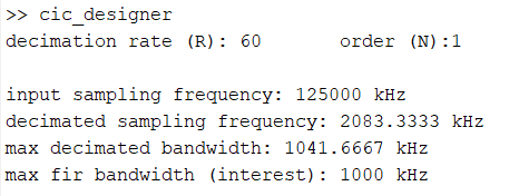
And here’s the response from the program:

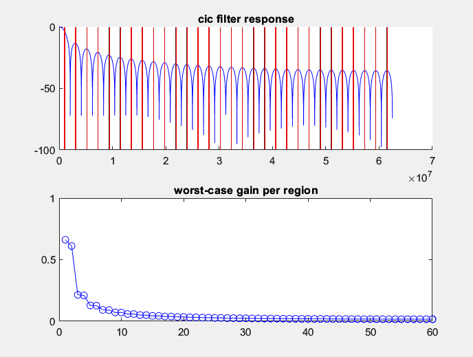
Region 1: 0 kHz -> 1041.6667 kHz  :: -3.5841 (worst)
Region 2: 1041.6667 kHz -> 2083.3333 :: -4.2791 (worst)
Region 3: 2083.3333 kHz -> 3125 kHz  :: -13.3568 (worst)
Region 4: 3125 kHz -> 4166.6667 :: -13.5879 (worst)
Region 5: 4166.6667 kHz -> 5208.3333 kHz  :: -17.8249 (worst)
Region 6: 5208.3333 kHz -> 6250 :: -17.963 (worst)
...
Region 59: 60416.6667 kHz -> 61458.3333 kHz  :: -35.577 (worst)
Region 60: 61458.3333 kHz -> 62500 :: -35.5775 (worst)

This is telling us something important — if we CIC decimate by a factor of 60, the worst-case attenuation in Region 1 (from 0 → 1.042 MHz) will be -3.581 dB (0.662 gain). This is pretty bad, since the signal we are interested in has been partially filtered out already.

The following attenuations will be aliased back into Region 1. For example, whatever the frequency components in Region 2 (from 1.042 MHz → 2.083 MHz) will be attenuated by -4.279 dB (0.611 gain), before it aliases itself back into Region 1.

Overall, this isn’t great. The positive we gained from such a high decimation rate means that our filter that will come after this down-sampler will be cheaper since the frequency range has been reduced … but we’ve tampered with the signal and haven’t fully dealt with aliasing.

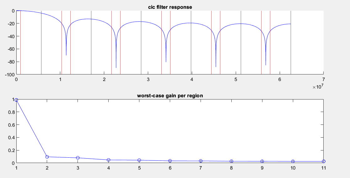
So let’s trade off one for another, and increase the frequency range which means reducing the decimation rate. Plugging in R = 11, N = 1:

decimation rate (R): 11       order (N):1
 
input sampling frequency: 125000 kHz
decimated sampling frequency: 11363.6364 kHz
max decimated bandwidth: 5681.8182 kHz
max fir bandwidth (interest): 1000 kHz
 
Region 1: 0 kHz -> 5681.8182 kHz  :: -0.11001 (worst)
Region 2: 5681.8182 kHz -> 11363.6364 :: -20.3228 (worst)
Region 3: 11363.6364 kHz -> 17045.4545 kHz  :: -21.8137 (worst)
Region 4: 17045.4545 kHz -> 22727.2727 :: -26.415 (worst)
Region 5: 22727.2727 kHz -> 28409.0909 kHz  :: -27.0948 (worst)
Region 6: 28409.0909 kHz -> 34090.9091 :: -29.4797 (worst)
Region 7: 34090.9091 kHz -> 39772.7273 kHz  :: -29.8582 (worst)
Region 8: 39772.7273 kHz -> 45454.5455 :: -31.1805 (worst)
Region 9: 45454.5455 kHz -> 51136.3636 kHz  :: -31.3799 (worst)
Region 10: 51136.3636 kHz -> 56818.1818 :: -31.9831 (worst)
Region 11: 56818.1818 kHz -> 62500 kHz  :: -32.0459 (worst)

And this is a lot better! Now the gain in the passband is at worst -0.1101 dB (0.987 gain), but the attenuation is very strong for the Regions 2 and onwards, and almost no higher-frequency components alias back in.

Overall, we’ve made our work down the line a little more difficult because any filter after such a decimator now needs to work over the 0 → 11.364 MHz range, but at least we are strongly attenuating everything outside of the signal-of-interest-passband.

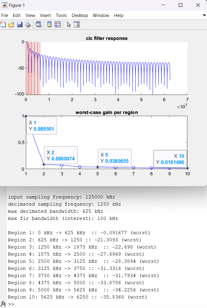
Here’s another quick plot for a CIC for a signal-of-interest with maximum bandwidth of 100 kHz. It’s important to design such down-samplers ahead of time, because any filters sitting downstream of them will need to know the rate at which they will sample at (to calculate their coefficients):

Finally, here’s the code:

clear
plot_db = true;
plot_gain_interval_db = false;
v_scale = true;

% sampling and outputs
fS = 125e6;  % source clock
max_fir_bandwidth = 100e3;

% parameters

N = 1;
R = 100;
Rlimit = 10;
M = 1;
disp(['decimation rate (R): ' num2str(R) '       order (N):' num2str(N) ])
disp(' ')
disp(['input sampling frequency: ' num2str(fS*10^(-3)) ' kHz'])
disp(['decimated sampling frequency: ' num2str(fS/(R^N)*10^(-3)) ' kHz'])
decim_bandwidth = (0.5*fS)/(R^N);
diff_bandwidth = decim_bandwidth - max_fir_bandwidth;
disp(['max decimated bandwidth: ' num2str(decim_bandwidth*10^(-3)) ' kHz'])
disp(['max fir bandwidth (interest): ' num2str(max_fir_bandwidth * 10^-3) ' kHz'])
disp(' ');

if (diff_bandwidth < 0)
    disp('ERROR: max fir bandwidth must be less than decimated bandwidth');
else
    cic = dsp.CICDecimator(R,M,N);
    gains = [];
    ax1 = subplot(2,1,1); % Create the first subplot for the frequency response
    ax2 = subplot(2,1,2); % Create the second subplot for gains

    % Plot the frequency response in the first subplot
    axes(ax1);
    title('cic filter response');
    [H, w] = freqz(cic);
    X = w/(2*pi) * fS;
    if (v_scale); Y = 1/R^N * abs(H); else; Y = abs(H); end
    if (plot_db); Y = 20*log10(Y); end
    
    % plotting
    hold on
    plot(X, Y, 'Color', 'blue');

    % folds and lines
    for n=1:Rlimit
        bandwidth_fold = decim_bandwidth * n;
        if (mod(n, 2) == 1)
    
            
            Q = interp1(X,Y,bandwidth_fold-diff_bandwidth);
            if (isnan(Q))
                Rlimit = n - 1;
                break
            end
            xline(bandwidth_fold-diff_bandwidth, 'Color', 'red');
            disp(['Region ' num2str(n) ': ' num2str((bandwidth_fold-decim_bandwidth)*10^-3) ' kHz -> ' ...
                  num2str(bandwidth_fold * 10^-3) ' kHz  :: ' num2str(Q) ' (worst)'])
            if plot_gain_interval_db gains(n) = Q; else gains(n) = 10^(Q/20); end
            
            xline(bandwidth_fold);
           
            Q = interp1(X,Y,bandwidth_fold+diff_bandwidth);
            if (isnan(Q))
                Rlimit = n;
                break
            end
            xline(bandwidth_fold+diff_bandwidth, 'Color', 'red');
            disp(['Region ' num2str(n+1) ': ' num2str(bandwidth_fold * 10^-3) ' kHz -> ' ...
                  num2str((bandwidth_fold+decim_bandwidth)*10^-3) ' :: ' num2str(Q) ' (worst)'])
            if plot_gain_interval_db gains(n+1) = Q; else gains(n+1) = 10^(Q/20); end            
            
        end
    end
    
    hold off
    
    % Plot the gains in the second subplot
    axes(ax2);
    
    ngains = 1:Rlimit;
    plot(ngains, gains, 'b-o');
    if (~plot_gain_interval_db)
        ylim([0, 1])
    end
    xlim([1, inf])
    title('worst-case gain per region');
end